在R中可视化-一种k-表示聚类发育基因表达数据集

Question

我可以看到很多关于这个话题的帖子，但是没有一个能解决这个问题。如果我错过了一个相关的答案，很抱歉。我有一个大型的蛋白质表达数据集，像这样的样本，如: rep1_0hr，rep1_16hr，rep1_24hr，rep1_48hr，rep1_72hr……

以及行中的2000+蛋白。换句话说，每个样本都是一个不同的开发时间点。

如果感兴趣，则原始数据集是R中的mulvey2015包中的“pRolocdata”，我将其转换为RStudio中的SummarizedExperiment对象。

我首先对数据(一个assay()的SummarizedExperiment数据集)进行k-均值聚类，以获得12个集群：

k_mul <- kmeans(scale(assay(mul)), centers = 12, nstart = 10)

然后：

summary(k_mul)

产生了预期的产出。

我希望可视化看起来像这样，样本在x轴上，表达式在y轴上。这些图看起来就像使用ggplot中的facet_wrap()生成的：

​

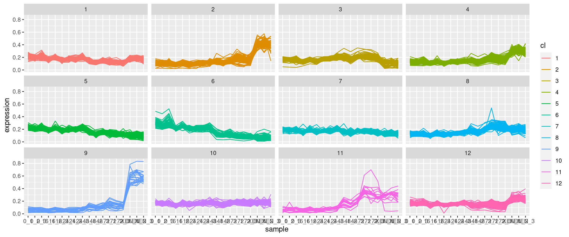
对于ggplot，需要将数据作为带有单个蛋白质集群标识列的数据提供。此外，数据需要采用长格式。我尝试过旋转(pivot_longer)原始数据集，但是当然有大量的数据点。此外，我贴出的图片显示，在任何一幅图中，彩色线条的数量都小于蛋白质的总数，这表明数据集上可能首先出现了维数减少，但我不确定。到目前为止，我一直在运行没有降维的kmeans算法。我能得到如何制作这个情节的指导吗？

Answer 1

以下是我试图扭转这一阴谋的企图：

library(pRolocdata)
library(dplyr)
library(tidyverse)
library(magrittr)
library(ggplot2)

mulvey2015 %>%
  Biobase::assayData() %>%
  magrittr::extract2("exprs") %>%
  data.frame(check.names = FALSE) %>%
  tibble::rownames_to_column("prot_id") %>%
  mutate(.,
         cl = kmeans(select(., -prot_id),
                     centers = 12,
                     nstart = 10) %>%
           magrittr::extract2("cluster") %>%
           as.factor()) %>%
  pivot_longer(cols = !c(prot_id, cl),
               names_to = "Timepoint",
               values_to = "Expression") %>%
  ggplot(aes(x = Timepoint, y = Expression, color = cl)) +
  geom_line(aes(group = prot_id)) +
  facet_wrap(~ cl, ncol = 4)

至于您的问题，除非pivot_longer无法在键中找到唯一的组合或与数据类型转换相关的问题，否则它通常是很有性能的。该地块可通过以下方式加以改善：

Timepoint

• changing

• 对geom_lines的alpha参数进行了调整(例如alpha = 0.5)，以提供线条密度的概念，为

• 找到一个很好的缩写和顺序，用于geom_lines axis.text.x取向

​

​

Answer 2

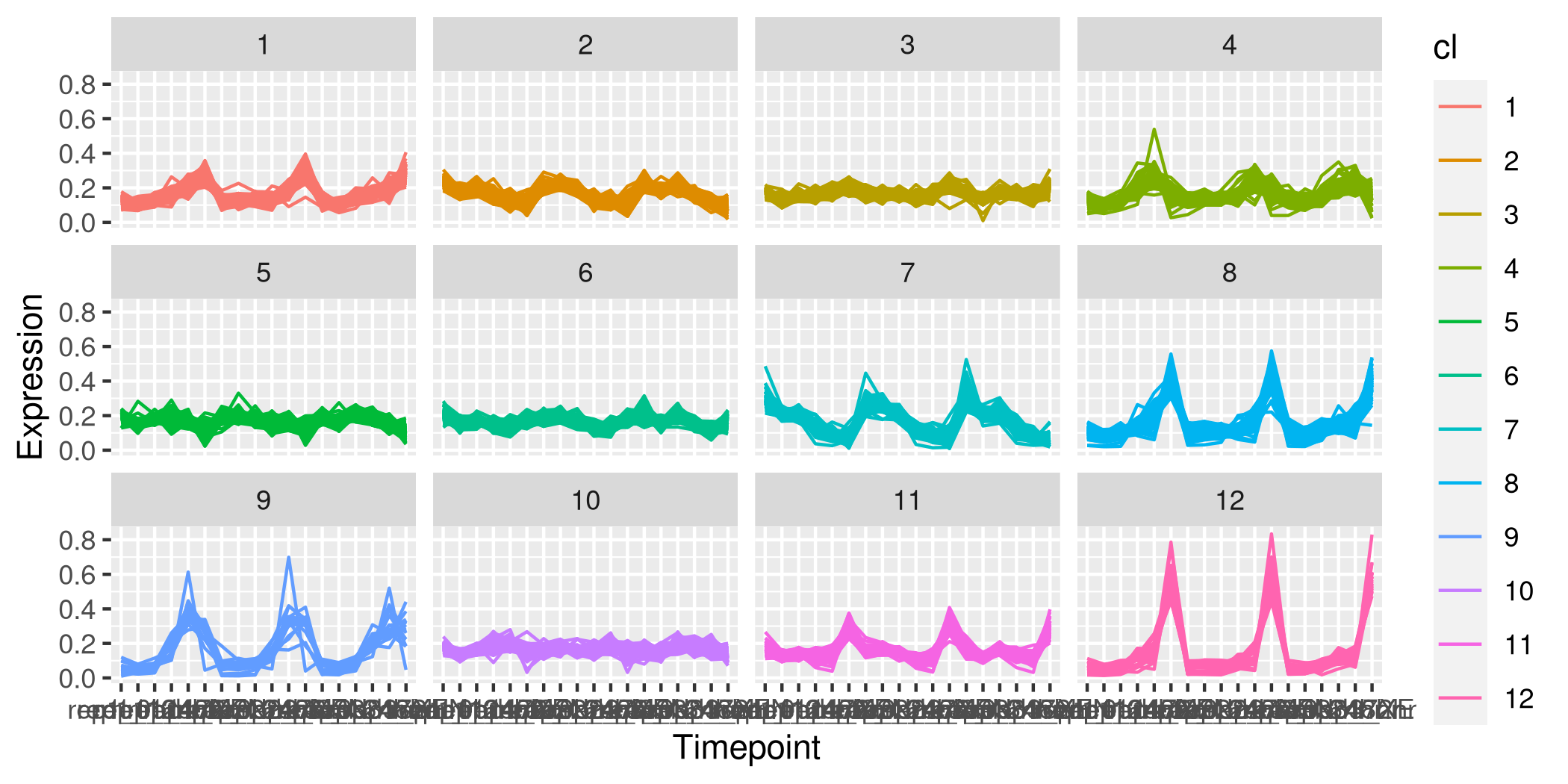
这是我自己的，非常相似的解决方案以上。

dfsa_mul <- data.frame(scale(assay(mul)))
dfsa_mul2 <- rownames_to_column(dfsa_mul, "protID")

将kmeans $cluster列添加到dfsa_mul2数据框架中。只在执行clus后将pivot_longer更改为一个因子

dfsa_mul2$clus <- ksa_mul$cluster
dfsa_mul2 %>% 
  pivot_longer(cols = -c("protID", "clus"),
               names_to = "samples",
               values_to = "expression") %>% 
ggplot(aes(x = samples, y = expression, colour = factor(clus))) +
  geom_line(aes(group = protID)) +
  facet_wrap(~ factor(clus))

这将生成一系列与@sbarbit发布的图表相同的情节。