LMS波束形成Julia规划

Question

我一直试图实现一个简单的LMS自适应波束形成代码。由于我没有Matlab许可证，所以我决定使用Julia，因为它们非常相似。为了使基本代码正常工作，我实现了MVRD波束形成示例，该示例在Matlabs网站上找到(我现在似乎找不到链接)。然后，我使用链接https://teaandtechtime.com/adaptive-beamforming-with-lms/使LMS运行。

我现在的代码是

using Plots
using LinearAlgebra

# Source: https://teaandtechtime.com/adaptive-beamforming-with-lms/

M   = 20;        # Number of Array Elements.
N   = 200;       # Number of Signal Samples.
n   = 1:N;       # Time Sample Index Vector.
c   = 3*10^8;    # Speed of light
f   = 2.4*10^9;  # Frequency [Hz]
lambda = c/f;    # Incoming Signal Wavelength in [m].
d = lambda/2;    # Interelement Distance in [m].
SNR    = 20;     # Target SNR in dBs.
phi_s  = 0;      # Target azimuth angle in degrees.
phi_i1 = 20;     # Interference angle in degrees.
phi_i2 = -30;    # Interference angle in degrees.
phi_i3 = 50;     # Interference angle in degrees.
INR1   = 35;     # Interference #1 INR in dBs.
INR2   = 70;     # Interference #2 INR in dBs.
INR3   = 50;     # Interference #3 INR in dBs.

u_s    = (d/lambda)*sin(phi_s*pi/180);   # Normalized Spatial Frequency of the Target signal.
u_int1 = (d/lambda)*sin(phi_i1*pi/180);  # Normalized Spatial Frequency of the Interferer #1.
u_int2 = (d/lambda)*sin(phi_i2*pi/180);  # Normalized Spatial Frequency of the Interferer #2.
u_int3 = (d/lambda)*sin(phi_i3*pi/180);  # Normalized Spatial Frequency of the Interferer #3.

tau_s  = (d/c)*sin(phi_s*pi/180);     # Time delay of the Target signal.
tau1   = (d/c)*sin(phi_i1*pi/180);    # Time delay of the Interferer #1.
tau2   = (d/c)*sin(phi_i2*pi/180);    # Time delay of the Interferer #2.
tau3   = (d/c)*sin(phi_i3*pi/180);    # Time delay of the Interferer #3.

# Target Signal definition.
s = zeros(ComplexF64,M,N)
v_s = exp.(-1im*2*pi*u_s*collect(0:M-1))/sqrt(M);  # Target Steering Vector.
for k=1:N
    s[:,k] = 10^(SNR/20)*v_s;  # Amplitude of Target Signal Generation.
end

# The uncorrelated unit power thermal noise samples with a Gaussian
# distribution are generated by:
w = (randn(M,N)+1im*randn(M,N))/sqrt(2)

# The interference [1iammer] vectors are generated by:
v_i1 = exp.(-1im*2*pi*u_int1*collect(0:M-1))/sqrt(M)
i_x1 = 10^(INR1/20)*v_i1*(randn(1,N)+1im*randn(1,N))/sqrt(2)

v_i2 = exp.(-1im*2*pi*u_int2*collect(0:M-1))/sqrt(M)
i_x2 = 10^(INR2/20)*v_i2*(randn(1,N)+1im*randn(1,N))/sqrt(2)

v_i3 = exp.(-1im*2*pi*u_int3*collect(0:M-1))/sqrt(M)
i_x3 = 10^(INR3/20)*v_i3*(randn(1,N)+1im*randn(1,N))/sqrt(2)

# The three signals are added to produce the overall array signal.
x = s + i_x1 + i_x2 + i_x3 + w

# Run LMS algorithm
mu = 0.001;                 # LMS step size
a = ones(ComplexF64,M);     # Complex weights
S = zeros(ComplexF64,M);    # Complex weights

ts = 1/(N*f);               # sample time
 
for k = 1:N
    d = cos(2*pi*f*k*ts);       # Reference Signal
    S = a.*x[:,k];
    y = sum(S);
    global e = conj(d) - y;
    println(e)
    global a += mu*x[:,k]*e;    # next weight calculation
end

println(a)
# Array Response
Nsamples1 = 3*10^4
angle1        = -90:180/Nsamples1:90-180/Nsamples1
LMS_Beam_Pat  = zeros(ComplexF64,Nsamples1)

for k = 1:Nsamples1
    u = (d/lambda)*sin(angle1[k]*pi/180)
    v = exp.(-1im*2*pi*u*collect(0:M-1))/sqrt(M); # Azimuth Scanning Steering Vector.
    LMS_Beam_Pat[k]  = a'*v;
end

# Plot the corresponding Beampatterns.
display(plot(angle1,10*log10.(abs.(LMS_Beam_Pat).^2),xlims=(-90,90),ylims=(-100,0)))

sleep(10)

# PolardB plot
display(plot(angle1*pi/180,10*log10.(abs.(LMS_Beam_Pat).^2), proj=:polar, lims=(-80,0)))

sleep(10)

LMS代码不会收敛(它会发散)，我也不知道为什么。我也不明白参考信号位和它如何是不同的目标转向矢量。也许对一般概念作一些澄清会很有帮助。我是新来的波束形成，我的背景是在根解决等。

下面是从Matlab示例中重写的已工作的Julia代码。它几乎与上面的代码相同，但没有LMS部分。

using Plots
using LinearAlgebra

M   = 20;        # Number of Array Elements.
N   = 200;       # Number of Signal Samples.
n   = 1:N;       # Time Sample Index Vector.
c   = 3*10^8;    # Speed of light
f   = 2.4*10^9;  # Frequency [Hz]
lambda = c/f;    # Incoming Signal Wavelength in [m].
d = lambda/2;    # Interelement Distance in [m].
SNR    = 20;     # Target SNR in dBs.
phi_s  = 0;      # Target azimuth angle in degrees.
phi_i1 = 20;     # Interference angle in degrees.
phi_i2 = -30;    # Interference angle in degrees.
phi_i3 = 50;     # Interference angle in degrees.
INR1   = 35;     # Interference #1 INR in dBs.
INR2   = 70;     # Interference #2 INR in dBs.
INR3   = 50;     # Interference #3 INR in dBs.

u_s    = (d/lambda)*sin(phi_s*pi/180);   # Normalized Spatial Frequency of the Target signal.
u_int1 = (d/lambda)*sin(phi_i1*pi/180);  # Normalized Spatial Frequency of the Interferer #1.
u_int2 = (d/lambda)*sin(phi_i2*pi/180);  # Normalized Spatial Frequency of the Interferer #2.
u_int3 = (d/lambda)*sin(phi_i3*pi/180);  # Normalized Spatial Frequency of the Interferer #3.

tau_s  = (d/c)*sin(phi_s*pi/180);     # Time delay of the Target signal.
tau1   = (d/c)*sin(phi_i1*pi/180);    # Time delay of the Interferer #1.
tau2   = (d/c)*sin(phi_i2*pi/180);    # Time delay of the Interferer #2.
tau3   = (d/c)*sin(phi_i3*pi/180);    # Time delay of the Interferer #3.

# Target Signal definition.
s = zeros(ComplexF64,M,N)
v_s = exp.(-1im*2*pi*u_s*collect(0:M-1))/sqrt(M);  # Target Steering Vector.
for k=1:N
    s[:,k] = 10^(SNR/20)*v_s;  # Amplitude of Target Signal Generation.
end

# The uncorrelated unit power thermal noise samples with a Gaussian
# distribution are generated by:
w = (randn(M,N)+1im*randn(M,N))/sqrt(2)

# The interference [1iammer] vectors are generated by:
v_i1 = exp.(-1im*2*pi*u_int1*collect(0:M-1))/sqrt(M)
i_x1 = 10^(INR1/20)*v_i1*(randn(1,N)+1im*randn(1,N))/sqrt(2)

v_i2 = exp.(-1im*2*pi*u_int2*collect(0:M-1))/sqrt(M)
i_x2 = 10^(INR2/20)*v_i2*(randn(1,N)+1im*randn(1,N))/sqrt(2)

v_i3 = exp.(-1im*2*pi*u_int3*collect(0:M-1))/sqrt(M)
i_x3 = 10^(INR3/20)*v_i3*(randn(1,N)+1im*randn(1,N))/sqrt(2)

#The three signals are added to produce the overall array signal.
x = s + i_x1 + i_x2 + i_x3 + w

iplusn = i_x1 + i_x2 + i_x3 + w

# Calculation of the i+n autocorrelation matrix.
R_ipn = 10^(INR1/10)*(v_i1*v_i1') + 10^(INR2/10)*(v_i2*v_i2') + 10^(INR3/10)*(v_i3*v_i3') + I

InvR = inv(R_ipn)

# Calculate the Beam Patterns.

# MVDR Optimum Beamformer computed for a phi_s = 0 deg.
c_opt = InvR*v_s/(v_s'*InvR*v_s); 

# Spatial Matched Filter | Steering Vector Beamformer Eq. (11.2.16).
c_mf = v_s

Nsamples1 = 3*10^4
angle1        = -90:180/Nsamples1:90-180/Nsamples1
Opt_Beam_Pat  = zeros(ComplexF64,Nsamples1)
Conv_Beam_Pat = zeros(ComplexF64,Nsamples1)

for k = 1:Nsamples1
    u = (d/lambda)*sin(angle1[k]*pi/180)
    v = exp.(-1im*2*pi*u*collect(0:M-1))/sqrt(M); # Azimuth Scanning Steering Vector.
    Opt_Beam_Pat[k]  = c_opt'*v
    Conv_Beam_Pat[k] = c_mf'*v
end

# Plot the corresponding Beampatterns.
plot(angle1,10*log10.(abs.(Conv_Beam_Pat).^2))
display(plot!(angle1,10*log10.(abs.(Opt_Beam_Pat).^2),xlims=(-90,90),ylims=(-100,0)))

sleep(10)

# PolardB plot
display(plot(angle1*pi/180,10*log10.(abs.(Opt_Beam_Pat).^2), proj=:polar, lims=(-80,0)))

sleep(10)

# Calculate the SINR loss factor for the Optimum Beamformer:
Nsamples = 3*10^4;  # The resolution must be very fine to reveal the true depth of the notches.
Lsinr_opt = zeros(ComplexF64,Nsamples,1);
Lsinr_mf  = zeros(Nsamples,1);
SNR0 = M*10^(SNR/10);
angle = -90:180/Nsamples:90-180/Nsamples;

for k=1:Nsamples
    v = exp.(-1im*pi*collect(0:M-1)*sin(angle[k]*pi/180))/sqrt(M); # Azimuth Scanning Steering Vector.
    c_mf = v;  # This is the spatial matched filter beamformer.
    Lsinr_opt[k] = v'*InvR*v;
    SINRout_mf = real(M*(10^(SNR/10))*(abs(c_mf'*v)^2)/(c_mf'*R_ipn*c_mf));
    Lsinr_mf[k] = SINRout_mf/SNR0;
end

plot(angle,10*log10.(abs.(Lsinr_opt)),xlims=(-90,0));
display(plot!(angle,10*log10.(abs.(Lsinr_mf)),xlims=(-90,90),ylims=(-75,5)));

sleep(10)

Answer 1

一个好的做法是迭代地构建模拟。

人们应该意识到，当所有其他数据都在干扰时，自适应滤波器就会适应参考信号。数据与参考数据的相关性越强，就越难适应它。

因此，参考信号应该是你可以从传感器上的信号中过滤出来的信号。例如，它可以是它的非延迟版本，也可以是传感器获取的信号。

为了让事情更简单，我创建了一个真实信号的例子，根据传感器的不同，它基本上可以得到不同的延迟。

将延迟加到实信号中的最简单的方法是调整其解析信号的相位并取实信号。

然后，我们基本上有N信号和M样本，每个样本进入自适应滤波器，在M x N矩阵的每一行上应用一个内积。

我用MATLAB和Julia做了一个简单的模拟。

这是朱莉娅代码的结果：

​

​

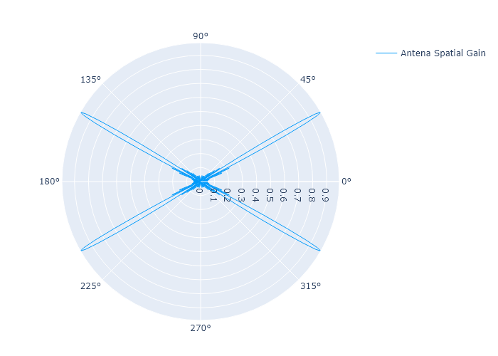
在上面，我们看到天线增益的目标信号来自30 [Deg]和干扰在[20.0; -35.0; 50.0]。

可以看出，该数组确实适应并在参考方向上具有~1增益，同时拒绝所有其他方向。

完整的代码可以在我的StackExchange信号处理Q81138 GitHub仓库上使用(查看SignalProcessing\Q81138文件夹)。