论文复现 | 第 05 章:回归分析与合成图——量化气候因果

论文复现 | 第 05 章:回归分析与合成图——量化气候因果

用户11172986
发布于 2026-04-24 19:35:25
发布于 2026-04-24 19:35:25
第 05 章:回归分析与合成图——量化气候因果
1. 科学背景
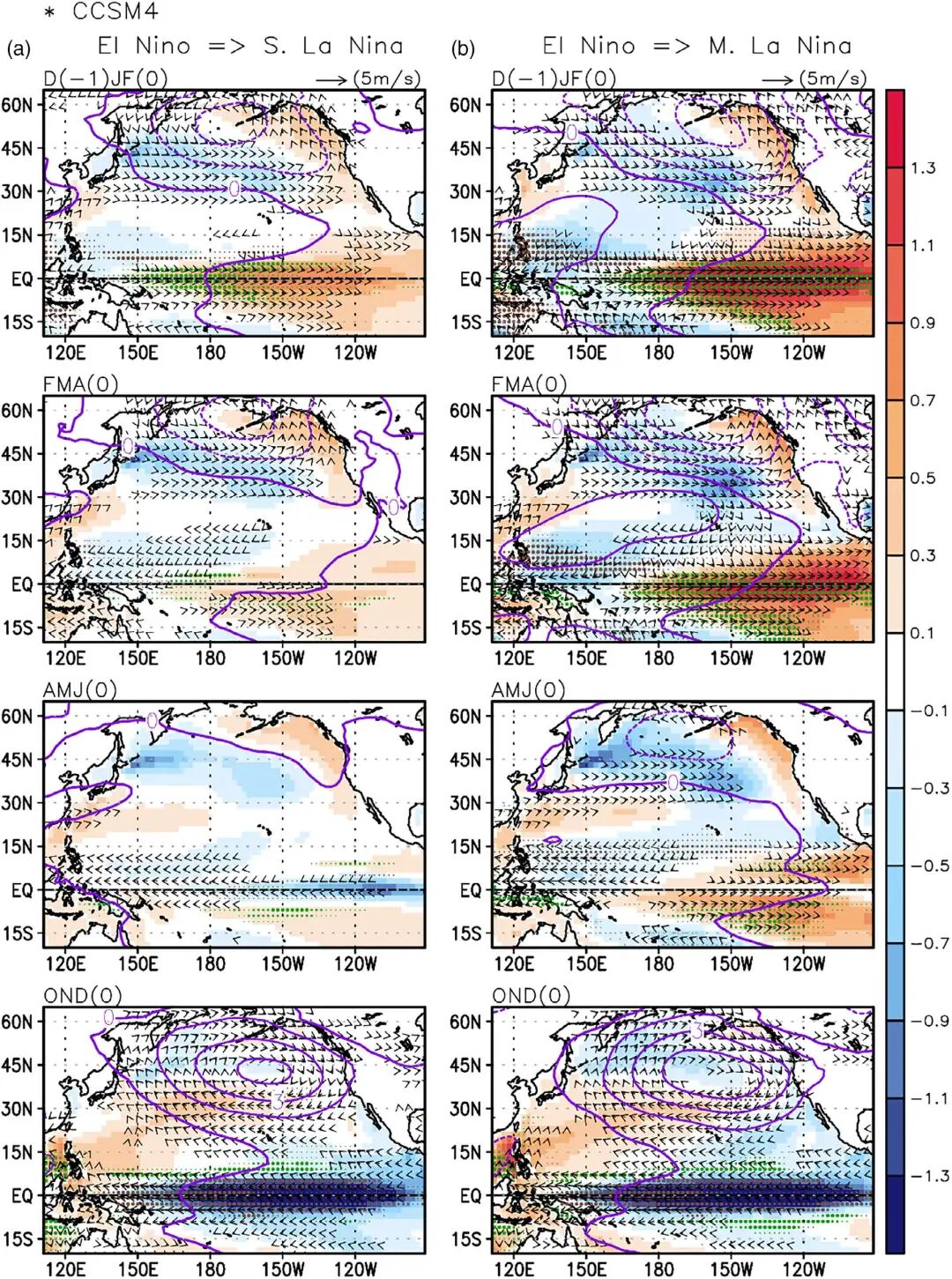
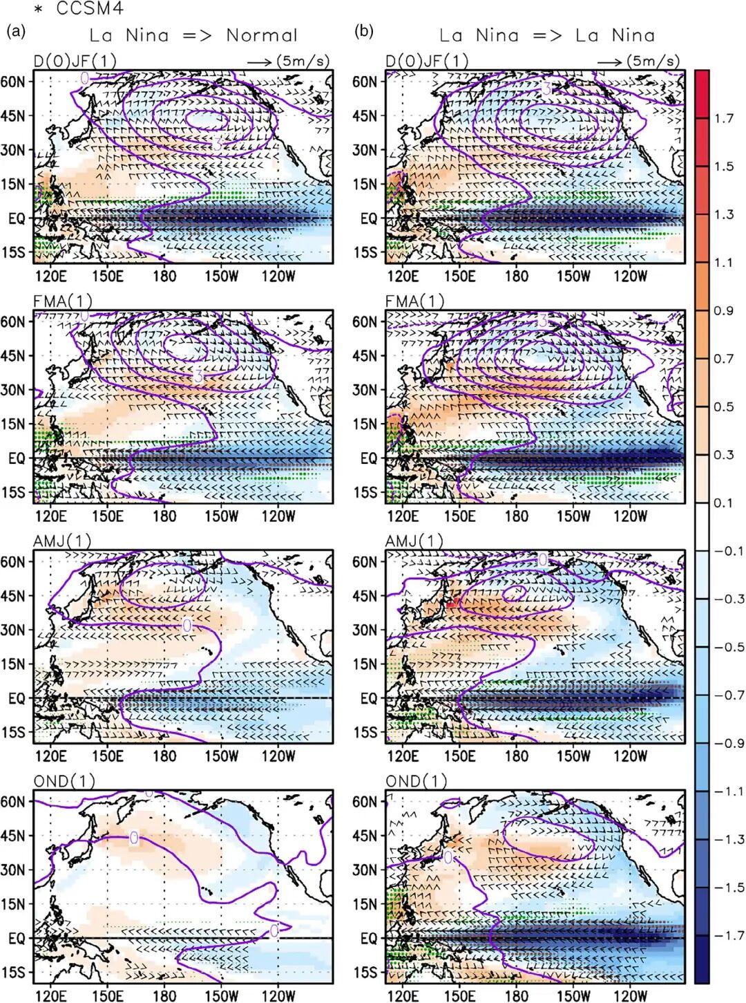
除了直接平均(合成),线性回归 (Linear Regression) 是量化一个变量(如 SSTA)如何影响另一个变量(如 SLP)最常用的统计工具。Figure 7 & 8 通过序列合成图详细展示了从厄尔尼诺转换到单年型/多年型拉尼娜的演变差异。
import xarray as xr
import numpy as np
import matplotlib.pyplot as plt
import cartopy.crs as ccrs
import cartopy.feature as cfeature
from scipy import stats
import warnings
warnings.filterwarnings('ignore')

# --- 配置 ---
DATA_DIR = r"./data"
SST_FILE = f"{DATA_DIR}/sst.mnmean.nc"
SLP_FILE = f"{DATA_DIR}/slp.mon.mean.nc"
UWND_FILE = f"{DATA_DIR}/uwnd.mon.mean.nc"
VWND_FILE = f"{DATA_DIR}/vwnd.mon.mean.nc"
PRATE_FILE = f"{DATA_DIR}/prate.mon.mean.nc"

SINGLE_YEAR_EVENTS = [1964, 1988, 1995, 2005]
MULTI_YEAR_EVENTS = [1949, 1954, 1970, 1973, 1998, 2007, 2010]
LON_RANGE = slice(100, 300)
LAT_RANGE = slice(70, -20)

CLIM_START, CLIM_END = '1981-01-01', '2010-12-31'
2. 核心函数:异常值、回归与合成
在气象数据分析中,我们经常需要对每个网格点执行回归,或者根据特定月份组合计算合成图。
def calculate_anomaly(ds, var_name):
    """计算月异常"""
    clim = ds.sel(time=slice(CLIM_START, CLIM_END)).groupby("time.month").mean("time")
    return (ds.groupby("time.month") - clim)[var_name]

def get_seasonal_composite(var, events, month_specs):
    """
    根据月份规格创建合成图
    month_specs: list of (year_offset, month) tuples
    """
    composites = []
    for year in events:
        monthly_data = []
        for y_off, m in month_specs:
            try:
                chunk = var.sel(time=f"{year+y_off}-{m:02d}-01", method='nearest')
                monthly_data.append(chunk.values)
            except: continue
        if monthly_data: composites.append(np.nanmean(monthly_data, axis=0))
    return np.nanmean(composites, axis=0) if composites elseNone
3. 面板绘图逻辑
我们将 SST (填色)、SLP (等值线)、风场 (矢量) 和降水 (打点) 结合在同一个地图面板中。
def plot_panel(ax, sst, slp, u, v, precip, title, lon, lat):
    ax.set_extent([100, 300, -20, 70], crs=ccrs.PlateCarree())
    ax.coastlines(linewidth=0.5)

    lon_g, lat_g = np.meshgrid(lon, lat)

    # SST 填色
    cf = ax.contourf(lon_g, lat_g, sst, levels=np.arange(-1.5, 1.6, 0.1), cmap='RdBu_r', extend='both', transform=ccrs.PlateCarree())

    # SLP 等值线
    if slp isnotNone:
        ax.contour(lon_g, lat_g, slp, levels=np.arange(0.5, 4, 0.5), colors='magenta', linewidths=0.6, transform=ccrs.PlateCarree())
        ax.contour(lon_g, lat_g, slp, levels=np.arange(-3.5, 0, 0.5), colors='magenta', linewidths=0.6, linestyles='--', transform=ccrs.PlateCarree())

    # 风场矢量
    skip = (slice(None, None, 4), slice(None, None, 4))
    ax.quiver(lon_g[skip], lat_g[skip], u[skip], v[skip], scale=60, width=0.003, transform=ccrs.PlateCarree())

    # 降水打点 (简化展示)
    if precip isnotNone:
        mask = np.abs(precip) > 0.5e-6
        ax.scatter(lon_g[mask], lat_g[mask], s=1, c='green', alpha=0.3, transform=ccrs.PlateCarree())

    ax.set_title(title, fontsize=9, fontweight='bold')
    return cf
4. 复现图与原图对比
Figure 7
复现图
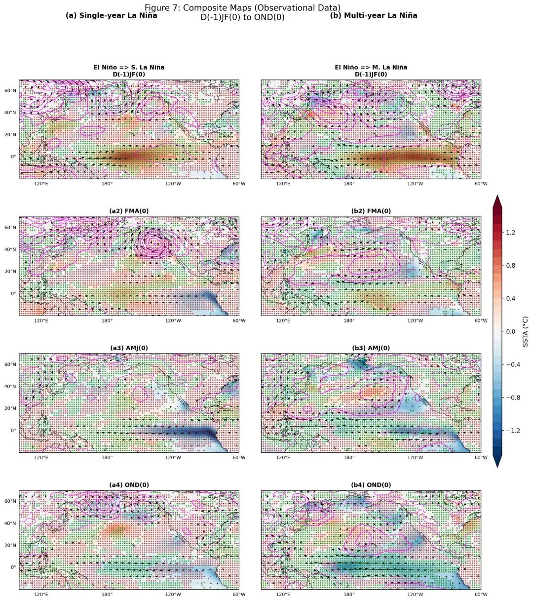
figure7_reproduction
figure7_reproduction
原图
page10_img1
page10_img1
Figure 8
复现图
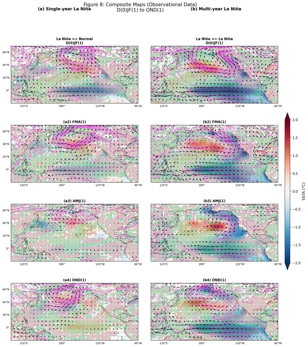
figure8_reproduction
figure8_reproduction
原图
page11_img1
page11_img1
完整代码 fig7
本文参与 腾讯云自媒体同步曝光计划,分享自微信公众号。
原始发表:2026-04-04,如有侵权请联系 cloudcommunity@tencent.com 删除
评论
登录后参与评论
推荐阅读
目录
腾讯云开发者

Copyright © 2013 - 2026 Tencent Cloud. All Rights Reserved. 腾讯云 版权所有
深圳市腾讯计算机系统有限公司 ICP备案/许可证号:粤B2-20090059 ![]() 粤公网安备44030502008569号
粤公网安备44030502008569号
腾讯云计算(北京)有限责任公司 京ICP证150476号 | 京ICP备11018762号