代码实战 | FNL 数据处理与 MCAPE 计算教程

代码实战 | FNL 数据处理与 MCAPE 计算教程

用户11172986
发布于 2026-04-24 19:28:24
发布于 2026-04-24 19:28:24
前些时间看气象家园有人问 gs 怎么画 fnl 的 cape,说实话 gs 已经还给老师,咱们用比较熟悉的 python 写一个教程。本教程介绍如何使用 Python 处理 FNL (Final Analysis) GRIB2 数据,计算最大对流有效位能 (MCAPE),并绘制全球/区域分布图。
主要内容
- FNL 数据格式与结构
- 使用 xarray + cfgrib 读取 GRIB2 数据
- 使用 wrf-python 计算 MCAPE
- 使用 meteva 绘制中国/世界地图
- 完整代码实现
1. 环境准备
所需库
pip install xarray cfgrib wrf-python matplotlib cartopy meteva
导入库
#!/usr/bin/env python3
import argparse
import sys
from pathlib import Path

import numpy as np
import xarray as xr
from wrf import cape_2d
import matplotlib.pyplot as plt
import cartopy.crs as ccrs
import cartopy.feature as cfeature
from meteva.base.tool.plot_tools import add_china_map_2basemap
2. FNL 数据结构
FNL (Final Analysis) 是 NCEP 的全球分析数据,包含:
2.1 数据层次
层次类型 | 说明 | 主要变量 |
|---|---|---|
等压面层 (isobaricInhPa) | 3D 数据,33个气压层 | 温度、比湿、位势高度、风场 |
地面层 (surface) | 2D 数据 | 地面气压、地形、CAPE、CIN |
2.2 气压层分布
从 1000 hPa 到 1 hPa,共 33 层:
[1000, 975, 950, 925, 900, 850, 800, 750, 700, 650, 600, 550, 500,
 450, 400, 350, 300, 250, 200, 150, 100, 70, 50, 40, 30, 20, 15,
 10, 7, 5, 3, 2, 1] hPa
2.3 关键变量说明
# 变量名映射表(用于自动识别不同命名规范的变量)
PRESSURE_LEVEL_KEYS = ["isobaricInhPa", "level", "pressure", "lev"]
TEMP_KEYS = ["t", "temperature", "T"]
Q_KEYS = ["q", "qv", "specific_humidity", "QV", "qvapor"]
GHT_KEYS = ["gh", "ght", "geopotential_height", "HGT", "z"]
SURFACE_PS_KEYS = ["sp", "ps", "psfc", "surface_pressure", "PRES"]
TERRAIN_KEYS = ["orog", "terrain", "HGT_surface", "z_surface", "geopotential_height"]
3. 读取 FNL 数据
FNL GRIB2 文件需要分层读取:
def open_fnl_datasets(file_path):
    """
    读取 FNL GRIB2 文件

    Parameters:
        file_path: FNL GRIB2 文件路径

    Returns:
        ds_pl: 等压面数据 (3D)
        ds_sfc: 地面数据 (2D)
    """
    # 读取等压面数据 (3D)
    ds_pl = xr.open_dataset(
        file_path,
        engine="cfgrib",
        backend_kwargs={"filter_by_keys": {"typeOfLevel": "isobaricInhPa"}},
    )

    # 读取地面数据 (2D)
    ds_sfc = xr.open_dataset(
        file_path,
        engine="cfgrib",
        backend_kwargs={"filter_by_keys": {"typeOfLevel": "surface"}},
    )

    return ds_pl, ds_sfc

# 使用示例
ds_pl, ds_sfc = open_fnl_datasets("fnl_20220101_00_00.grib2")
3.1 查看数据变量
# 等压面变量(3D)
print("等压面变量:", list(ds_pl.data_vars))
# 输出: ['gh', 't', 'r', 'q', 'w', 'wz', 'u', 'v', 'absv', 'o3mr']

# 地面变量(2D)
print("地面变量:", list(ds_sfc.data_vars))
# 输出包含: ['sp', 'orog', 't', 'cape', 'cin', ...]

# 其中 orog 是地形数据,单位为米
4. MCAPE 计算原理
4.1 什么是对流有效位能 (CAPE)
CAPE 是衡量大气对流不稳定能量的重要指标,表示气块从自由对流高度 (LFC) 抬升到平衡高度 (EL) 所获得的浮力能量。
4.2 什么是 MCAPE
MCAPE (Maximum CAPE) 是最大对流有效位能,与常规 CAPE 的区别:
类型 | 计算方法 | 用途 |
|---|---|---|
CAPE | 从地面或特定层抬升 | 单点对流潜力 |
MCAPE | 寻找最低3000m内最大theta-e的气块 | 最大可能对流潜力 |
4.3 wrf.cape_2d 算法
wrf.cape_2d(pres_hpa, tkel, qv, height, terrain, psfc_hpa, ter_follow, meta=True)
算法步骤:
- 在最低 3000m 内寻找最大 theta-e 的高度层
- 以该层为中心,计算 500m 厚度的气块平均温湿特性
- 使用该"最大"气块计算 MCAPE、MCIN、LCL、LFC
输入参数:
参数 | 单位 | 说明 |
|---|---|---|
pres_hpa | hPa | 全气压(3D) |
tkel | K | 温度(3D) |
qv | kg/kg | 水汽混合比(3D) |
height | m | 位势高度(3D) |
terrain | m | 地形高度(2D) |
psfc_hpa | hPa | 地面气压(2D) |
ter_follow | bool | 是否地形跟随坐标 |
输出 (4层):
return_val[0]= MCAPE [J/kg]return_val[1]= MCIN [J/kg]return_val[2]= LCL [m]return_val[3]= LFC [m]
5. 数据预处理
def pick_var(ds, candidates, label):
    """从数据集中自动识别变量"""
    for name in candidates:
        if name in ds.data_vars:
            return ds[name]
    raise KeyError(f"未找到{label}变量,候选: {candidates},当前变量: {list(ds.data_vars)}")

def pick_coord(ds, candidates, label):
    """从数据集中自动识别坐标"""
    for name in candidates:
        if name in ds.coords:
            return ds.coords[name]
    raise KeyError(f"未找到{label}坐标,候选: {candidates},当前坐标: {list(ds.coords)}")
5.1 单位转换与维度调整
def preprocess_data(ds_pl, ds_sfc):
    """
    数据预处理:提取变量、单位转换、维度调整
    """
    # 1. 提取变量
    t = pick_var(ds_pl, TEMP_KEYS, "温度")          # 温度 [K]
    q = pick_var(ds_pl, Q_KEYS, "比湿")            # 比湿 [kg/kg]
    ght = pick_var(ds_pl, GHT_KEYS, "位势高度")    # 位势高度 [m]
    ps = pick_var(ds_sfc, SURFACE_PS_KEYS, "地面气压")  # 地面气压 [Pa]
    cape = pick_var(ds_sfc, SURFACE_PS_KEYS, "地面气压")
    # 提取地形数据
    try:
        terrain = pick_var(ds_sfc, TERRAIN_KEYS, "地形")
    except KeyError:
        terrain = xr.zeros_like(ps)

    # 2. 单位转换
    # 温度:确保单位为 K
    if t.max() < 100:
        t = t + 273.15

    # 构造 3D 气压场并转换为 hPa
    pres_coord = pick_coord(ds_pl, PRESSURE_LEVEL_KEYS, "气压层")
    pres_3d, _ = xr.broadcast(pres_coord, t)
    pres_hpa = pres_3d  # 已经是 hPa

    # 地面气压:Pa -> hPa
    ps_hpa = ps / 100.0

    # 3. 垂直层顺序调整(从地面向上:1000 -> 1 hPa)
    # 如果第一层气压小于最后一层(如 1hPa < 1000hPa),需要翻转
    if pres_hpa.isel(isobaricInhPa=0).values.mean() < pres_hpa.isel(isobaricInhPa=-1).values.mean():
        print("检测到气压层为高空到地面,正在进行垂直翻转...")
        pres_hpa = pres_hpa.isel(isobaricInhPa=slice(None, None, -1))
        t = t.isel(isobaricInhPa=slice(None, None, -1))
        q = q.isel(isobaricInhPa=slice(None, None, -1))
        ght = ght.isel(isobaricInhPa=slice(None, None, -1))

    return pres_hpa, t, q, ght, terrain, ps_hpa
6. 计算 MCAPE
def calculate_mcape(pres_hpa, t, q, ght, terrain, ps_hpa):
    """
    使用 wrf-python 计算 MCAPE

    Parameters:
        pres_hpa: 3D 气压场 [hPa]
        t: 3D 温度 [K]
        q: 3D 比湿 [kg/kg]
        ght: 3D 位势高度 [m]
        terrain: 2D 地形高度 [m]
        ps_hpa: 2D 地面气压 [hPa]

    Returns:
        mcape: 2D MCAPE 场 [J/kg]
        mcin: 2D MCIN 场 [J/kg]
        lcl: 2D LCL 场 [m]
        lfc: 2D LFC 场 [m]
    """
    print("正在计算 MCAPE (这可能需要一点时间)...")

    cape_result = cape_2d(
        pres_hpa,
        t,
        q,
        ght,
        terrain,
        ps_hpa,
        ter_follow=False,  # FNL 是等压面坐标,非地形跟随
        meta=True
    )

    # 提取结果
    mcape = cape_result[0]  # MCAPE
    mcin = cape_result[1]   # MCIN
    lcl = cape_result[2]    # LCL
    lfc = cape_result[3]    # LFC

    return mcape, mcin, lcl, lfc
7. 使用 meteva 绘制地图
meteva 是一个气象数据处理和可视化库,提供了方便的中国/世界地图绘制功能。
7.1 add_china_map_2basemap 函数
add_china_map_2basemap(ax, name="province", edgecolor='k', lw=0.5, encoding='gbk', grid0=None)
name 参数选项:
值 | 说明 | 适用场景 |
|---|---|---|
"world" | 世界地图 | 全球范围绘图 |
"nation" | 国界 | 中国区域 |
"province" | 省界 | 中国区域 |
"river" | 河流 | 中国区域 |
"county" | 县界 | 精细区域 |
def plot_mcape(lon, lat, mcape, extent, output_file, title="MCAPE"):
    """
    绘制 MCAPE 分布图

    Parameters:
        lon: 经度坐标
        lat: 纬度坐标
        mcape: MCAPE 数据
        extent: 绘图范围 [lon_min, lon_max, lat_min, lat_max]
        output_file: 输出文件名
        title: 图表标题
    """
    # 创建图形
    fig = plt.figure(figsize=(16, 10))
    ax = fig.add_subplot(1, 1, 1, projection=ccrs.PlateCarree())

    # 设置范围
    is_global = extent == [-180, 180, -90, 90]
    if is_global:
        ax.set_global()
    else:
        ax.set_extent(extent, crs=ccrs.PlateCarree())

    # 绘制填色图
    levels = [0, 100, 250, 500, 750, 1000, 1500, 2000, 3000, 4000]
    cf = ax.contourf(lon, lat, mcape, levels=levels, cmap="Spectral_r",
                     extend="max", transform=ccrs.PlateCarree())

    # 添加地图要素
    try:
        if is_global:
            # 全球范围使用 world 参数
            add_china_map_2basemap(ax, name="world", edgecolor='black', lw=0.8, encoding='gbk', grid0=None)
            print("成功加载 meteva 世界地图")
        else:
            # 区域范围使用中国地图要素
            add_china_map_2basemap(ax, name="river", edgecolor='dodgerblue', lw=0.5, encoding='gbk', grid0=None)
            add_china_map_2basemap(ax, name="nation", edgecolor='black', lw=1.0, encoding='gbk', grid0=None)
            add_china_map_2basemap(ax, name="province", edgecolor='gray', lw=0.5, encoding='gbk', grid0=None)
            print("成功加载 meteva 中国地图")
    except Exception as e:
        # 如果 meteva 加载失败,使用 cartopy 作为备用
        ax.coastlines(resolution='110m'if is_global else'50m', lw=0.8)
        ax.add_feature(cfeature.BORDERS, linestyle=':', alpha=0.5)
        print(f"提示: meteva 地图加载失败 ({e}),已切换至 cartopy 海岸线。")

    # 添加网格线
    gl = ax.gridlines(draw_labels=True, linestyle="--", alpha=0.5)
    gl.top_labels = False
    gl.right_labels = False

    # 添加色标和标题
    plt.colorbar(cf, ax=ax, label="MCAPE (J/kg)", orientation='vertical', pad=0.02, shrink=0.7)
    plt.title(f"Maximum Convective Available Potential Energy (MCAPE)\n{title}",
              loc="left", fontsize=10)

    # 保存图片
    plt.savefig(output_file, dpi=200, bbox_inches="tight")
    print(f"绘图成功,输出文件: {output_file}")
    plt.show()
8. 完整流程整合
def main(file_path, output_file, extent):
    """
    主函数:完整的 MCAPE 计算和绘图流程

    Parameters:
        file_path: FNL GRIB2 文件路径
        output_file: 输出图片路径
        extent: 绘图范围 [lon_min, lon_max, lat_min, lat_max]
    """
    file_path = Path(file_path)
    ifnot file_path.exists():
        raise FileNotFoundError(f"未找到文件: {file_path}")

    # 1. 加载数据
    print("步骤 1: 加载 FNL 数据...")
    ds_pl, ds_sfc = open_fnl_datasets(str(file_path))

    # 2. 数据预处理
    print("步骤 2: 数据预处理...")
    pres_hpa, t, q, ght, terrain, ps_hpa = preprocess_data(ds_pl, ds_sfc)

    # 3. 计算 MCAPE
    print("步骤 3: 计算 MCAPE...")
    mcape, mcin, lcl, lfc = calculate_mcape(pres_hpa, t, q, ght, terrain, ps_hpa)

    # 4. 获取经纬度坐标
    lon = pick_coord(ds_pl, ["longitude", "lon"], "经度")
    lat = pick_coord(ds_pl, ["latitude", "lat"], "纬度")

    # 5. 经度处理(从 0-360 转换到 -180-180)
    if lon.max() > 181:
        lon_data = lon.values.copy()
        lon_idx = lon_data > 180
        lon_data[lon_idx] -= 360
        lon = xr.DataArray(lon_data, dims=lon.dims, coords=lon.coords, attrs=lon.attrs)
        # 重新排序以防绘图断裂
        sort_idx = np.argsort(lon.values)
        lon = lon.isel(longitude=sort_idx)
        mcape = mcape.isel(longitude=sort_idx)

    # 6. 绘图
    print("步骤 4: 绘制地图...")
    plot_mcape(lon, lat, mcape, extent, output_file, title=f"Source: {file_path.name}")

    print("\n完成!")
    return mcape, mcin, lcl, lfc
9. 运行示例
# 示例 1: 绘制全球 MCAPE 分布
mcape_global, mcin_global, lcl_global, lfc_global = main(
    file_path="/home/mw/project/fnl_20220101_00_00.grib2",
    output_file="mcape_global.png",
    extent=[-180, 180, -90, 90]
)
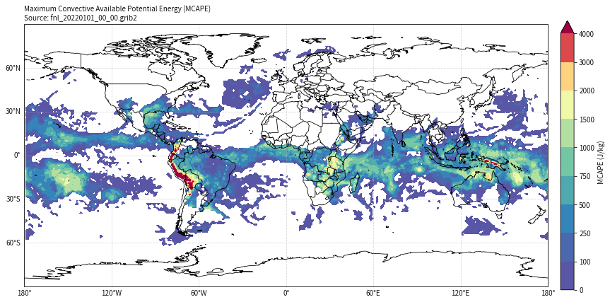
image
image
# 示例 2: 绘制中国区域 MCAPE 分布
mcape_china, mcin_china, lcl_china, lfc_china = main(
    file_path="/home/mw/project/fnl_20220101_00_00.grib2",
    output_file="mcape_china.png",
    extent=[70, 140, 15, 55]
)
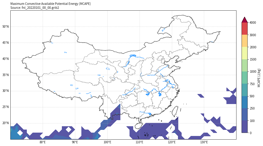
image
image
10. 结果分析
10.1 全球 MCAPE 分布特征
从全球 MCAPE 分布图可以观察到:
区域 | MCAPE 特征 | 原因 |
|---|---|---|
热带地区 (赤道附近) | 高值 (>2000 J/kg) | 高温高湿,对流活跃 |
亚马逊盆地 | 极高值 (>3000 J/kg) | 热带雨林,水汽充足 |
非洲中部 | 高值 (1500-2500 J/kg) | 热带草原气候 |
西太平洋暖池 | 高值 (>2000 J/kg) | 海温高,蒸发强 |
中高纬度 | 低值 (<500 J/kg) | 温度低,对流抑制 |
极地地区 | 接近 0 | 极冷干燥 |
沙漠地区 | 低值 | 干燥缺水 |
10.2 中国区域 MCAPE 特征
- 华南地区:冬季 MCAPE 较低(<500 J/kg)
- 南海区域:相对较高(500-1000 J/kg)
- 青藏高原:地形影响,MCAPE 分布复杂
那么顺带画一下fnl自带的cape
def read_fnl_cape(ds_sfc):
    """
    从 FNL 地面层数据中读取自带的 CAPE 和 CIN

    Parameters:
        ds_sfc: FNL 地面层数据集

    Returns:
        cape: 对流有效位能 [J/kg]
        cin: 对流抑制 [J/kg]
    """
    # FNL 中 CAPE 的变量名可能是 'cape' 或类似名称
    cape_keys = ["cape", "CAPE", "convective_available_potential_energy"]
    cin_keys = ["cin", "CIN", "convective_inhibition"]

    cape = pick_var(ds_sfc, cape_keys, "CAPE")
    cin = pick_var(ds_sfc, cin_keys, "CIN")

    return cape, cin

   # ============================================
   # 绘制 FNL 自带的 CAPE
   # ============================================

def plot_fnl_cape(lon, lat, cape, extent, output_file, title="FNL CAPE"):
    """
    绘制 FNL 自带的 CAPE 分布图

    Parameters:
        lon: 经度坐标
        lat: 纬度坐标
        cape: CAPE 数据 (来自FNL文件)
        extent: 绘图范围 [lon_min, lon_max, lat_min, lat_max]
        output_file: 输出文件名
        title: 图表标题
    """
    # 创建图形
    fig = plt.figure(figsize=(16, 10))
    ax = fig.add_subplot(1, 1, 1, projection=ccrs.PlateCarree())

    # 设置范围
    is_global = extent == [-180, 180, -90, 90]
    if is_global:
        ax.set_global()
    else:
        ax.set_extent(extent, crs=ccrs.PlateCarree())

    # 绘制填色图 - CAPE 使用与 MCAPE 相同的色标
    levels = [0, 100, 250, 500, 750, 1000, 1500, 2000, 3000, 4000]
    cf = ax.contourf(lon, lat, cape, levels=levels, cmap="Spectral_r",
                    extend="max", transform=ccrs.PlateCarree())

    # 添加地图要素
    try:
        if is_global:
            add_china_map_2basemap(ax, name="world", edgecolor='black', lw=0.8, encoding='gbk')
        else:
            add_china_map_2basemap(ax, name="river", edgecolor='dodgerblue', lw=0.5, encoding='gbk')
            add_china_map_2basemap(ax, name="nation", edgecolor='black', lw=1.0, encoding='gbk')
            add_china_map_2basemap(ax, name="province", edgecolor='gray', lw=0.5, encoding='gbk')
    except Exception as e:
        ax.coastlines(resolution='110m'if is_global else'50m', lw=0.8)
        ax.add_feature(cfeature.BORDERS, linestyle=':', alpha=0.5)

    # 添加网格线
    gl = ax.gridlines(draw_labels=True, linestyle="--", alpha=0.5)
    gl.top_labels = False
    gl.right_labels = False

    # 添加色标和标题
    plt.colorbar(cf, ax=ax, label="CAPE (J/kg)", orientation='vertical', pad=0.02, shrink=0.7)
    plt.title(f"Convective Available Potential Energy (CAPE) from FNL\n{title}",
                loc="left", fontsize=10)

    # 保存图片
    plt.savefig(output_file, dpi=200, bbox_inches="tight")
    print(f"绘图成功,输出文件: {output_file}")
    plt.show()

   # ============================================
   # 主函数:读取并绘制 FNL 自带的 CAPE
   # ============================================

def plot_fnl_cape_main(file_path, output_file, extent):
    """
    主函数:读取 FNL 自带的 CAPE 并绘图

    Parameters:
        file_path: FNL GRIB2 文件路径
        output_file: 输出图片路径
        extent: 绘图范围 [lon_min, lon_max, lat_min, lat_max]
    """
    file_path = Path(file_path)
    ifnot file_path.exists():
        raise FileNotFoundError(f"未找到文件: {file_path}")

    # 1. 加载数据
    print("步骤 1: 加载 FNL 数据...")
    ds_pl, ds_sfc = open_fnl_datasets(str(file_path))

    # 2. 读取 FNL 自带的 CAPE
    print("步骤 2: 读取 FNL 自带的 CAPE...")
    cape, cin = read_fnl_cape(ds_sfc)

    # 3. 获取经纬度坐标
    lon = pick_coord(ds_pl, ["longitude", "lon"], "经度")
    lat = pick_coord(ds_pl, ["latitude", "lat"], "纬度")

    # 4. 经度处理(从 0-360 转换到 -180-180)
    if lon.max() > 181:
        lon_data = lon.values.copy()
        lon_idx = lon_data > 180
        lon_data[lon_idx] -= 360
        lon = xr.DataArray(lon_data, dims=lon.dims, coords=lon.coords, attrs=lon.attrs)
        sort_idx = np.argsort(lon.values)
        lon = lon.isel(longitude=sort_idx)
        cape = cape.isel(longitude=sort_idx)

    # 5. 绘图
    print("步骤 3: 绘制 CAPE 地图...")
    plot_fnl_cape(lon, lat, cape, extent, output_file, title=f"Source: {file_path.name}")

    print("\n完成!")
    return cape, cin

   # ============================================
   # 使用示例
   # ============================================

#    示例 1: 绘制全球 CAPE 分布
cape_global, cin_global = plot_fnl_cape_main(
    file_path="fnl_20220101_00_00.grib2",
    output_file="fnl_cape_global.png",
    extent=[-180, 180, -90, 90]
)

#    示例 2: 绘制中国区域 CAPE 分布
#    cape_china, cin_china = plot_fnl_cape_main(
#        file_path="fnl_20220101_00_00.grib2",
#        output_file="fnl_cape_china.png",
#        extent=[70, 140, 15, 55]
#    )
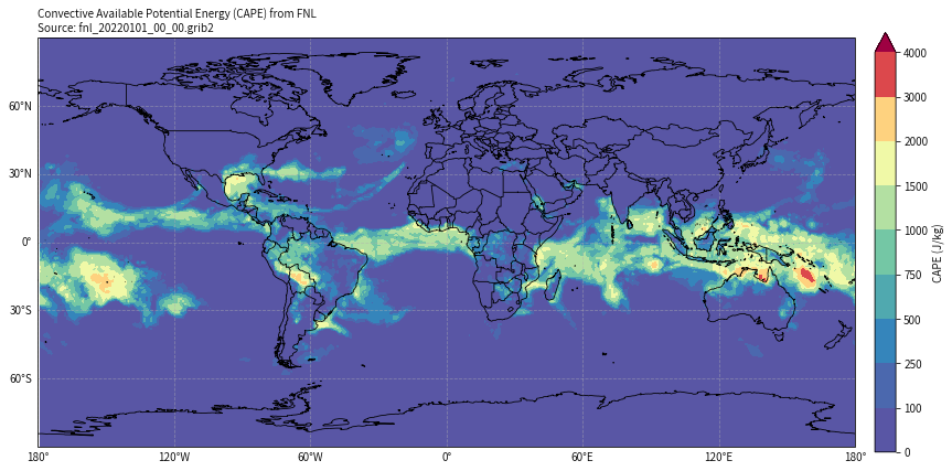
image
image
11. 常见问题与解决方案
Q1: cfgrib 读取时出现 DatasetBuildError
原因:不同变量的气压层数不一致
解决:这是正常现象,cfgrib 会自动跳过不匹配的变量,不影响主要变量读取。
Q2: 经度范围是 0-360,如何转换?
lon_data = lon.values.copy()
lon_data[lon_data > 180] -= 360
lon = xr.DataArray(lon_data, dims=lon.dims, coords=lon.coords)
Q3: 垂直层顺序问题
注意:wrf-python 要求气压层从地面向上排列(1000 -> 1 hPa)
if pres_hpa.isel(isobaricInhPa=0).values.mean() < pres_hpa.isel(isobaricInhPa=-1).values.mean():
    # 需要翻转(从高空向地面 -> 从地面向高空)
    pres_hpa = pres_hpa.isel(isobaricInhPa=slice(None, None, -1))
    t = t.isel(isobaricInhPa=slice(None, None, -1))
    # ... 其他变量同样处理
Q4: 气压单位问题
注意:wrf.cape_2d 函数要求:
pres_hpa和psfc_hpa的单位是 hPa- 不是 Pa(尽管文档可能有歧义)
Q5: meteva 地图加载失败
解决:代码已添加异常处理,自动切换到 cartopy 海岸线作为备用。
12. 扩展应用
12.1 计算其他对流参数
除了 MCAPE,cape_2d 还返回:
cape_result = cape_2d(pres_hpa, t, q, ght, terrain, ps_hpa, ter_follow=False, meta=True)

mcape = cape_result[0]  # 最大对流有效位能
mcin = cape_result[1]   # 最大对流抑制
lcl = cape_result[2]    # 抬升凝结高度
lfc = cape_result[3]    # 自由对流高度
12.2 批量处理多个时次
import glob

files = sorted(glob.glob("fnl_*.grib2"))
for file in files:
    output = file.replace(".grib2", "_mcape.png")
    main(file, output, extent=[70, 140, 15, 55])
12.3 制作动画
import imageio

images = []
for png_file in sorted(glob.glob("*_mcape.png")):
    images.append(imageio.imread(png_file))

imageio.mimsave("mcape_animation.gif", images, duration=0.5)
13. 参考资源
- wrf-python 文档
- xarray 文档
- cfgrib 文档
- meteva 文档
- NCEP FNL 数据说明
本文参与 腾讯云自媒体同步曝光计划,分享自微信公众号。
原始发表:2026-03-02,如有侵权请联系 cloudcommunity@tencent.com 删除
评论
登录后参与评论
推荐阅读
目录
腾讯云开发者

Copyright © 2013 - 2026 Tencent Cloud. All Rights Reserved. 腾讯云 版权所有
深圳市腾讯计算机系统有限公司 ICP备案/许可证号:粤B2-20090059 ![]() 粤公网安备44030502008569号
粤公网安备44030502008569号
腾讯云计算(北京)有限责任公司 京ICP证150476号 | 京ICP备11018762号