雷达系列 | 如何转换雷达三维球面坐标为经纬度坐标系

雷达系列 | 如何转换雷达三维球面坐标为经纬度坐标系

用户11172986
发布于 2026-04-24 19:22:19
发布于 2026-04-24 19:22:19
雷达系列 | 如何转换雷达三维球面坐标为经纬度坐标系
个人信息
公众号:气python风雨
关注我获取更多学习资料,第一时间收到我的Python学习资料,也可获取我的联系方式沟通合作
温馨提示
- 由于可视化代码过长隐藏,可点击运行Fork查看
- 若没有成功加载可视化图,点击运行可以查看
- ps:隐藏代码在【代码已被隐藏】所在行,点击所在行,可以看到该行的最右角,会出现个三角形,点击查看即可
前言
项目目标
- 理解球面坐标系(r, φ, θ)与投影坐标系之间的关系。
- 学习如何使用 wradlib.georef.polar.spherical_to_proj 函数将雷达数据从球面坐标转换为地图上的投影坐标。
- 掌握地球曲率及大气折射对雷达波束传播路径的影响
背景知识
- 极坐标系统通常用于描述雷达回波的位置,其中包含距离(r)、方位角(φ)和仰角(θ)。
- 投影坐标系统则是在平面上表示地理信息的一种方式,它考虑了地球的形状和大小。
- wradlib 是一个专门处理气象雷达数据的 Python 库。
函数说明
wradlib.georef.polar.spherical_to_proj 可以将给定的球面坐标转换为指定投影下的坐标。该函数考虑了随着仰角增加而缩短的大圆距离以及相应的高度增加。
参数
- r: 包含径向距离的数组。
- phi: 包含方位角的数组。
- theta: 包含仰角的数组。
- site: 雷达位置的经度/纬度坐标及其海拔高度。
- crs: 目标空间参考系统(投影),默认为 WGS84 (EPSG 4326)。
- re: 地球半径 [m],若未提供则根据给定纬度计算。
- ke: 修正因子,用来调整影响雷达波束传播的大气折射梯度,默认值 4/3 对大多数天气雷达波长是一个很好的近似。
返回
coords: 形状为 (..., 3) 的数组,包含了投影后的地图坐标。
简单示例
以下示例展示了如何从位于北纬48°东经9°的一个站点出发,沿不同方向(北、南、东、西)以大约1°的距离进行坐标转换:
import numpy as np
from wradlib.georef import polar

# 定义距离、方位角和仰角
r = np.array([0., 0., 111., 111., 111., 111.]) * 1000
az = np.array([0., 180., 0., 90., 180., 270.])
th = np.array([0., 0., 0., 0., 0., 0.5])

# 定义站点位置
csite = (9.0, 48.0, 0)

# 执行坐标转换
coords = polar.spherical_to_proj(r, az, th, csite)

# 输出结果
for coord in coords:
    print('{0:7.4f}, {1:7.4f}, {2:7.4f}'.format(*coord))
输出结果:
 9.0000, 48.0000,  0.0000
 9.0000, 48.0000,  0.0000
 9.0000, 48.9981, 725.7160
10.4872, 47.9904, 725.7160
 9.0000, 47.0017, 725.7160
 7.5131, 47.9904, 1694.2234
真实案例
import cartopy.crs as ccrs
import matplotlib.gridspec as gridspec
import matplotlib.pyplot as plt
import numpy as np

from metpy.calc import azimuth_range_to_lat_lon
from metpy.cbook import get_test_data
from metpy.io import Level3File
from metpy.plots import add_timestamp, colortables, USCOUNTIES
from metpy.units import units
# 打开雷达数据文件
name = '/home/mw/project/KOUN_SDUS54_N0QTLX_201305202016'
f = Level3File(name)
# 从文件对象中提取数据字典
datadict = f.sym_block[0][0]
# 根据文件指定的比例尺将数据转换为数组
data = f.map_data(datadict['data'])
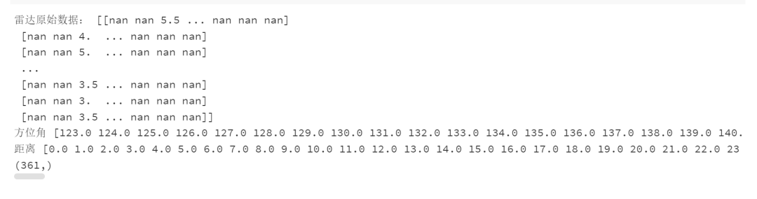
print("雷达原始数据:",data)
# 获取方位角和距离,并为其分配单位
az = units.Quantity(np.array(datadict['start_az'] + [datadict['end_az'][-1]]), 'degrees')
rng = np.linspace(0, f.max_range, data.shape[-1] + 1)*1000
print("方位角",az)
print("距离",rng)
print(az.shape)
# 从文件中提取中心经度和纬度
cent_lon = f.lon
cent_lat = f.lat
##设置参数
csite=(cent_lon,cent_lat,0)
theta= np.full(3, 361)
coords = polar.spherical_to_proj(rng, az, th, csite)
coords.shape
image
image
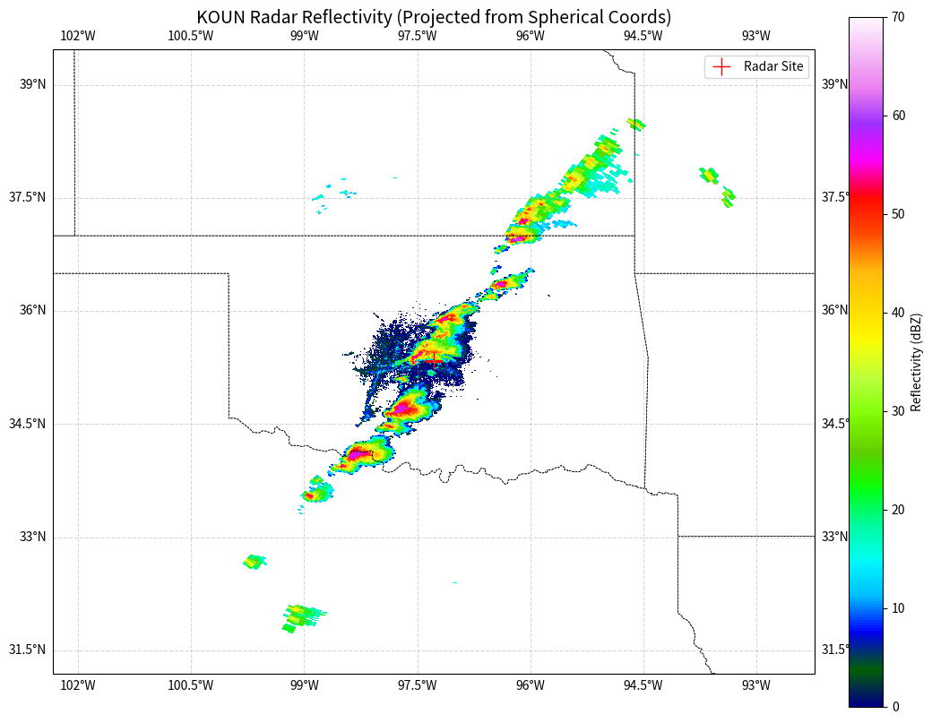
输出结果解释了各个点在投影坐标系中的位置,并且由于雷达波束并非沿着纬度圈而是沿着大圆路径传播,所以东西方向的坐标并不完全位于同一纬度上
在完成了 spherical_to_proj 的坐标转换后,我们得到了每个雷达门(gate)在地理空间中的实际经纬度(或投影坐标)。接下来,我们将使用 matplotlib 和 cartopy 将这些数据绘制出来,直观地观察雷达回波在地图上的分布,并验证地球曲率修正的效果。
为了演示,我们选取第一层数据进行绘图。
import matplotlib.pyplot as plt
import cartopy.crs as ccrs
import cartopy.feature as cfeature
import numpy as np

# 假设我们需要绘制第一个维度的结果(根据您的输出形状 (6, 361, 461, 3))
# 取出经度 (lon) 和 纬度 (lat)
# coords[..., 0] 是经度, coords[..., 1] 是纬度, coords[..., 2] 是高度
# 这里我们需要将数据降维以匹配 pcolormesh 的输入要求
# 假设 data 是 (361, 461) 的 2D 数组,我们取 coords 的第一个 slice
plot_coords = coords[0]
lons = plot_coords[:, :, 0]
lats = plot_coords[:, :, 1]

# 确保 data 的维度与 lons/lats 匹配
# 注意:pcolormesh 的坐标网格通常比数据多一行/一列,或者维度相同(取决于 shading='nearest' 或 'flat')
# 这里我们假设维度直接对应
plot_data = data  # 需确保 plot_data 是 2D 数组 (361, 461)
# 创建画布和投影
fig = plt.figure(figsize=(12, 10))
# 使用 PlateCarree 投影(等距圆柱投影),因为我们的 coords 是经纬度
ax = fig.add_subplot(1, 1, 1, projection=ccrs.PlateCarree())

# 添加地图特征
ax.add_feature(cfeature.COASTLINE, linewidth=1)
ax.add_feature(cfeature.BORDERS, linestyle=':')
ax.add_feature(cfeature.STATES, linestyle='--', linewidth=0.5) # 添加州界/省界
ax.gridlines(draw_labels=True, linestyle='--', alpha=0.5)

# 设置雷达回波的色标 (Reflectivity)
# 使用 MetPy 自带的色表,或者使用 standard 'pyart_HomeyerRainbow' 等
cmap = plt.get_cmap('gist_ncar')
cmap.set_bad('white', alpha=0) # 将 NaN 值设为透明

# 绘制数据
# transform=ccrs.PlateCarree() 告诉 cartopy 输入的 lons 和 lats 是经纬度数据
mesh = ax.pcolormesh(lons, lats, plot_data,
                     shading='auto',
                     cmap=cmap,
                     vmin=0, vmax=70, # 反射率因子通常在 0-70 dBZ 之间
                     transform=ccrs.PlateCarree())

# 添加色标
cbar = plt.colorbar(mesh, ax=ax, orientation='vertical', fraction=0.046, pad=0.04)
cbar.set_label('Reflectivity (dBZ)')

# 标记雷达站点位置
site_lon, site_lat, _ = csite
ax.plot(site_lon, site_lat, 'r+', markersize=15, transform=ccrs.PlateCarree(), label='Radar Site')
ax.legend()

# 设置标题
ax.set_title('KOUN Radar Reflectivity (Projected from Spherical Coords)', fontsize=14)

plt.show()
image
image
通过上述可视化代码,我们可以观察到以下现象:
- 扇形失真与地理对齐:雷达的原始数据是极坐标格式(方位角-距离),在普通的 plt.imshow 中会显示为矩形。经过 spherical_to_proj 转换并使用 pcolormesh 绘制后,图像正确地呈现为以雷达站点为中心的扇形,并能与地图上的地理边界(如海岸线、州界)精确吻合。
- 波束传播路径:如果您仔细观察远离雷达中心的区域,像素点的形状会发生微妙的变化。这是因为 wradlib 的转换函数考虑了地球曲率和大气折射(4/3 地球半径模型)。在高纬度或大范围扫描中,这种投影修正对于精确定位强对流天气至关重要。
总结
本项目通过 wradlib 库演示了气象雷达数据处理中的核心环节——坐标转换。理解球面坐标系 (r, ϕ, θ) 到地理投影坐标系的转换原理,是进行多源数据融合(如将雷达数据与卫星、地面站点或 WRF 模式数据叠加)的基础。
本文参与 腾讯云自媒体同步曝光计划,分享自微信公众号。
原始发表:2026-01-18,如有侵权请联系 cloudcommunity@tencent.com 删除
评论
登录后参与评论
推荐阅读
目录
腾讯云开发者

Copyright © 2013 - 2026 Tencent Cloud. All Rights Reserved. 腾讯云 版权所有
深圳市腾讯计算机系统有限公司 ICP备案/许可证号:粤B2-20090059 ![]() 粤公网安备44030502008569号
粤公网安备44030502008569号
腾讯云计算(北京)有限责任公司 京ICP证150476号 | 京ICP备11018762号