代码实战：如何使用Python绘制弯曲箭头的风场 (2.0版)

用户11172986

发布于 2026-04-24 19:19:58

630

文章被收录于专栏：气python风雨气python风雨

代码实战：如何使用Python绘制弯曲箭头的风场 (2.0版)

1. 项目简介

本项目展示了如何使用Python绘制弯曲箭头的风场可视化。相比传统的 quiver 图和 streamplot 图，弯曲箭头能够更直观、更优雅地展示风场的流动特征。

项目基于 GitHub 上的 curved-quivers 思想，通过自定义 modplot 模块中的 velovect 函数实现，并成功应用于 ERA5 气象数据的可视化中。

提示：需要将github的modplot.py代码下载并置于绘图文件夹中

2. 核心技术栈

Matplotlib: 基础绘图框架。
NumPy: 数值计算与网格处理。
Xarray: 处理 ERA5 气象数据。
Cartopy: 地理坐标投影与地图特征绘制。
Modplot: 自定义模块，包含核心的 velovect 函数（需将参考代码下载至绘图文件夹）。

3. 关键问题与解决方案

在实战过程中，直接调用 velovect 绘制 ERA5 风场时遇到了 IndexError 报错。

3.1 问题描述

报错信息如下：

IndexError: index 361 is out of bounds for axis 1 with size 361

原因：在 modplot.py 的 _integrate_rk12 函数内部调用的 interpgrid 函数中，当插值点接近或正好位于边界上时，计算 x + 1 或 y + 1 导致索引超出了数组的合法范围。

3.2 解决方案

修改 interpgrid 函数，使用 np.clip 对索引进行边界限制，确保所有索引均在有效范围内。

修改后的 interpgrid 函数代码：

def interpgrid(a, xi, yi):  
    """Fast 2D, linear interpolation on an integer grid"""

    Ny, Nx = np.shape(a)  

    if isinstance(xi, np.ndarray):  
        x = xi.astype(int)  
        y = yi.astype(int)  
        # 使用 np.clip 来确保 xn 和 yn 不会超出边界  
        xn = np.clip(x + 1, 0, Nx - 1)  
        yn = np.clip(y + 1, 0, Ny - 1)  
    else:  
        x = int(xi)  
        y = int(yi)  
        # 对于单个整数索引，直接进行边界检查  
        xn = min(x + 1, Nx - 1)  
        yn = min(y + 1, Ny - 1)  

    # 确保原始索引也在有效范围内  
    x = np.clip(x, 0, Nx - 1)  
    y = np.clip(y, 0, Ny - 1)  

    a00 = a[y, x]  
    a01 = a[y, xn]  
    a10 = a[yn, x]  
    a11 = a[yn, xn]  

    xt = xi - x  
    yt = yi - y  

    a0 = a00 * (1 - xt) + a01 * xt  
    a1 = a10 * (1 - xt) + a11 * xt  
    ai = a0 * (1 - yt) + a1 * yt  

    ifnot isinstance(xi, np.ndarray):  
        if np.ma.is_masked(ai):  
            raise TerminateTrajectory  

    return ai

改进点：

对数组类型的索引使用 np.clip 确保不越界。
对单个整数索引使用 min 函数限制最大值。
确保原始索引 x 和 y 也在有效范围内。

4. 代码实现示例

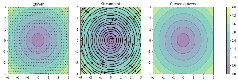
4.1 基础绘图对比 (Quiver vs Streamplot vs Curved Quivers)

import matplotlib.pyplot as plt
import numpy as np
from modplot import velovect

w = 3
Y, X = np.mgrid[-w:w:241j, -w:w:361j]

# 定义矢量场 U, V (旋转场)
U = -Y
V = X
W = np.sqrt(U**2 + V**2)

f, (ax1, ax2, ax3) = plt.subplots(1, 3, figsize=(15,4))

# 1. 传统 Quiver 图
s=10
ax1.quiver(X[::s,::s],Y[::s,::s],U[::s,::s],V[::s,::s])

# 2. Streamplot 流线图
ax2.streamplot(X,Y,U,V, color='k')

# 3. Curved Quivers 弯曲箭头图 (使用 velovect)
# 注意：此处需确保 modplot.py 已包含上述修复
grains = 15
tmp = np.linspace(-3, 3, grains)
xs = np.tile(tmp, grains)
ys = np.repeat(tmp, grains)
seed_points = np.array([list(xs), list(ys)])

velovect(ax3, X, Y, U, V, arrowstyle='fancy', scale=2.0, grains=15, color='k')
     
# 添加背景等值线
for ax in ax1, ax2, ax3:
 cs = ax.contourf(X,Y, W, cmap=plt.cm.viridis, alpha=0.5, zorder=-1)
 ax.set_xlim([-3,3])
 ax.set_ylim([-3,3])

ax1.set_title("Quiver")
ax2.set_title("Streamplot")
ax3.set_title("Curved quivers")

plt.colorbar(cs, ax=[ax1,ax2,ax3])  
plt.show()

image

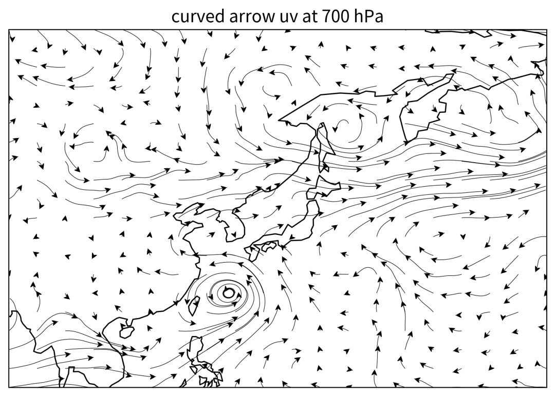
4.2 ERA5 实战数据可视化

import xarray as xr
import numpy as np
import matplotlib.pyplot as plt
import cartopy.crs as ccrs
import cartopy.feature as cfeature
from modplot import velovect

# 1. 读取数据
ds = xr.open_dataset('/home/mw/input/era58091/ERA5-2023-08_pl.nc')
# 选取 700hPa 等压面数据
u = ds['u'].sel(level=700, time='2023-08-02T00:00:00.000000000')
v = ds['v'].sel(level=700, time='2023-08-02T00:00:00.000000000') 

# 纬度反转以适配绘图习惯
u_reversed = u.sel(latitude=slice(None, None, -1))
v_reversed = v.sel(latitude=slice(None, None, -1))

# 构建网格
lon = u_reversed['longitude']
lat = u_reversed['latitude']
Lon, Lat = np.meshgrid(lon, lat)

# 2. 定义绘图函数
def plot_uv(u, v, lon, lat):
    fig = plt.figure(figsize=(8, 6), dpi=300)
    ax = plt.axes(projection=ccrs.PlateCarree())

    # 绘制弯曲箭头
    velovect(ax, lon, lat, u, v, 
             arrowstyle='fancy', 
             linewidth=0.4, 
             scale=8, 
             grains=20, 
             color='k')

    # 添加地理特征
    ax.add_feature(cfeature.COASTLINE)
    ax.set_title('Curved Arrow UV at 700 hPa', fontsize=14)
    ax.set_xlabel('Longitude', fontsize=12)
    ax.set_ylabel('Latitude', fontsize=12)

    plt.savefig('curved_arrow_wind.png', bbox_inches='tight')

# 3. 执行绘图
plot_uv(u_reversed.data, v_reversed.data, Lon, Lat)