WRF | 如何基于 wrfout 绘制艾玛图（Emagram）

用户11172986

发布于 2026-04-24 19:09:35

450

文章被收录于专栏：气python风雨气python风雨

WRF | 如何基于 wrfout 绘制艾玛图（Emagram）

前言

之前我们做过使用 WRF 绘制 TLNP 图的教程，有读者留言说想看看艾玛图的教程，遂写一下。

当然我是比较习惯看skew的，这种图还没怎么研究怎么看，希望有大佬赐教。

WRF 模式输出的 wrfout 文件蕴含丰富大气信息，但需有效工具提取分析。艾玛图（Emagram）是诊断大气热力结构的核心工具，能直观展示温、湿、风垂直廓线及对流能量。传统方法步骤繁琐，本文介绍基于 wrf-python 与 MetPy 的 Python 自动化方案，实现从数据提取到专业绘图的一键式流程，提升 WRF 结果分析效率。

环境准备

首先确保 MetPy ≥ 1.7（本文示例已升级至 1.7.1）。

pip install --upgrade metpy -i https://pypi.mirrors.ustc.edu.cn/simple/

完整绘图代码

import numpy as np
import matplotlib.pyplot as plt
from netCDF4 import Dataset
from wrf import getvar, ll_to_xy
import metpy.calc as mpcalc
from metpy.plots import Emagram          # ① 引入 Emagram
from metpy.units import units

# 1. 数据读取
ncfile = Dataset("/home/mw/input/typhoon9537/wrfout_d01_2019-08-08_19_00_00")
target_lat, target_lon = 25, 120.4

# 坐标转换与索引提取
xy = ll_to_xy(ncfile, target_lat, target_lon)
x_idx, y_idx = xy[0], xy[1]

# 提取变量
p  = getvar(ncfile, "pressure")[:, y_idx, x_idx] * units.hPa
tc = getvar(ncfile, "tc")[:, y_idx, x_idx]       * units.degC
td = getvar(ncfile, "td")[:, y_idx, x_idx]       * units.degC
u  = getvar(ncfile, "ua", units="kt")[:, y_idx, x_idx] * units.knots
v  = getvar(ncfile, "va", units="kt")[:, y_idx, x_idx] * units.knots

# 2. 计算参数
prof = mpcalc.parcel_profile(p, tc[0], td[0])
lcl_pressure, lcl_temperature = mpcalc.lcl(p[0], tc[0], td[0])
cape, cin = mpcalc.surface_based_cape_cin(p, tc, td)

# 3. 绘图 (Emagram)
fig = plt.figure(figsize=(9, 9))
emagram = Emagram(fig)                 # ② 无需 rotation

# 绘制层结曲线
emagram.plot(p, tc, 'r', linewidth=2, label='Temperature')
emagram.plot(p, td, 'g', linewidth=2, label='Dewpoint')
emagram.plot(p, prof, 'k', linewidth=2, linestyle='--', label='Parcel Path')

# 填充能量区
emagram.shade_cin(p, tc, prof, alpha=0.2)
emagram.shade_cape(p, tc, prof, alpha=0.2)

# 绘制风羽
interval = np.arange(0, len(p), 3)
emagram.plot_barbs(p[interval], u[interval], v[interval])

# 坐标轴与参考线
emagram.ax.set_ylim(1000, 200)
emagram.ax.set_xlim(-110, 40)
emagram.plot_dry_adiabats(alpha=0.25, color='orange')
emagram.plot_moist_adiabats(alpha=0.25, color='green')
emagram.plot_mixing_lines(alpha=0.25, color='purple')

# 标记 LCL
emagram.plot(lcl_pressure, lcl_temperature, 'ko', markerfacecolor='black')

# 标题
plt.title(f"Emagram @ ({target_lat}, {target_lon})", loc='left')
plt.title(f"CAPE: {cape.m:.0f} J/kg", loc='right')
plt.legend(loc='upper left')

plt.show()

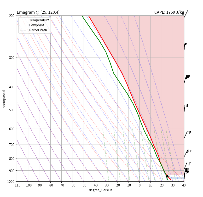
艾玛图

小结

本文以 wrfout 文件为基础，结合 wrf-python 进行数据提取与垂直插值，利用 MetPy 自动化绘制艾玛图。该方法统一了从原始数据到气象专业图表的处理流程，可快速生成含温度、露点、风场及 CAPE 区域的标准化图表。流程易于扩展至批量处理与时空对比，为 WRF 模拟的热力学诊断提供高效、可复现的解决方案。

本文参与腾讯云自媒体同步曝光计划，分享自微信公众号。

原始发表：2025-12-12，如有侵权请联系 cloudcommunity@tencent.com 删除

数据