空间转录组(1)—输入文件说明及数据读取
原创
空间转录组(1)—输入文件说明及数据读取
原创
sheldor没耳朵
发布于 2026-01-28 15:12:34
发布于 2026-01-28 15:12:34
空间转录组(1)—输入文件说明及数据读取
对于空转的数据分析,一直没有时间整理笔记,今天抽空写一篇,就从读取数据的开始吧。
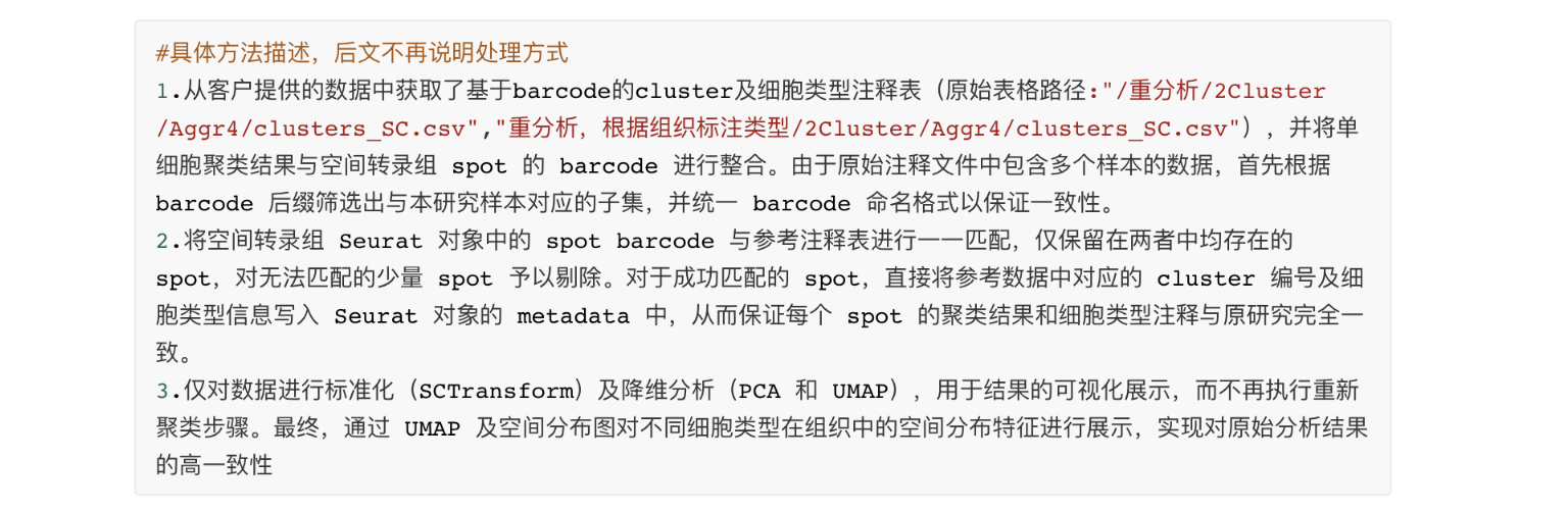
1.文件说明
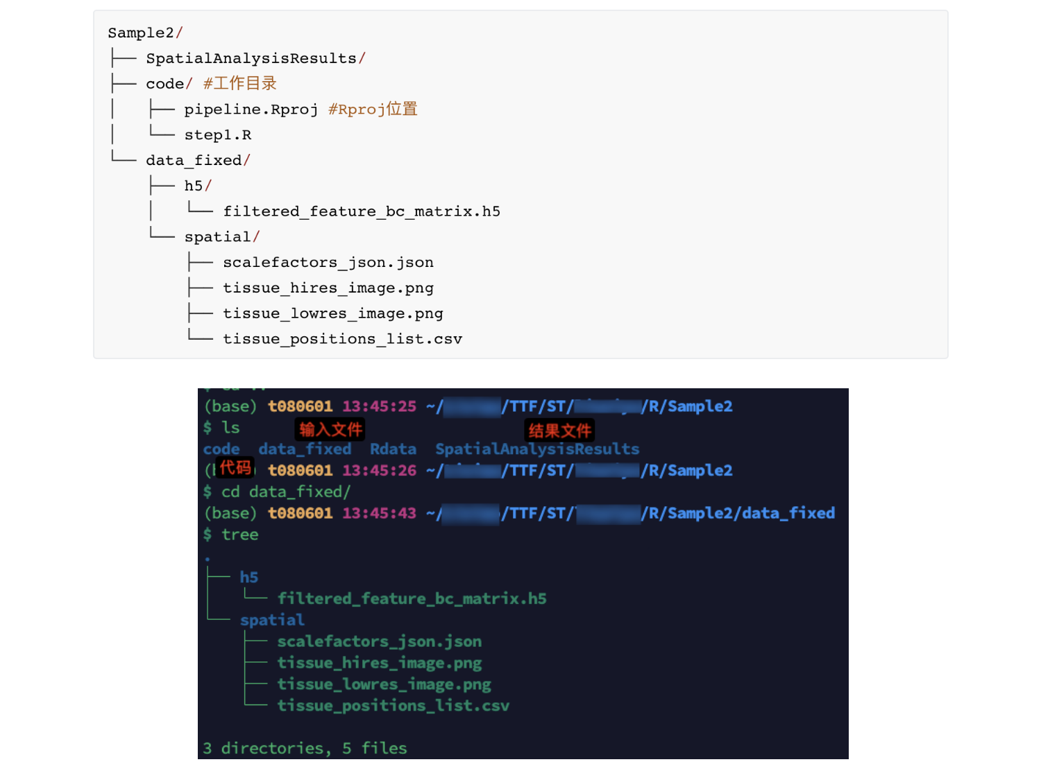
- 空转和单细胞一样,对于数据的读取有着严格的限制,如原始数据的文件名,文件位置等。对于单个样本(以样本名Sample2为例)的读取,需要以下的文件
- 文件介绍
- filtered_feature_bc_matrix.h5:存储经过初步过滤后的基因表达矩阵,记录每个空间 spot 上各基因的转录本计数信息,是后续分析的基础数据
- scalefactors_json.json:存储空间坐标与组织图像之间的缩放因子信息,用于保证空间坐标与图像的准确对齐

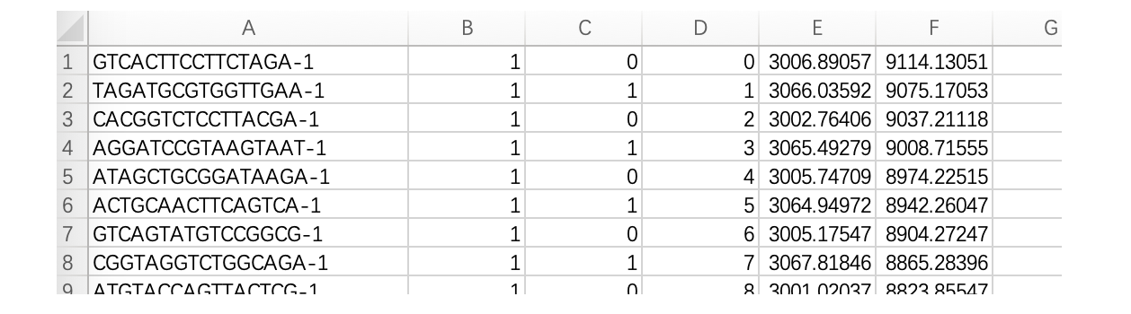
- tissue_positions_list.csv:记录每个 spot 的空间坐标信息,包括其在阵列中的位置及在组织图像中的像素坐标,用于将基因表达与空间位置对应(无列名,若加上列名,后续代码可能报错)
- tissue_lowres_image.png:组织切片的低分辨率图像,主要用于快速空间可视化展示(分析用,一定需要)
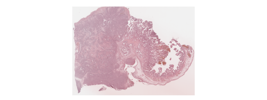
- tissue_hires_image.png:组织切片的高分辨率图像,用于精细的空间可视化和形态学展示(展示用,不一定需要)
- 目录层级
2.数据读取
- Seurat对象构建
rm(list = ls())
library(Seurat)        # 单细胞分析主包
library(ggplot2)       # 绘图
library(patchwork)     # 多图拼接
library(dplyr)         # 数据处理
library(Rfast2)        # 快速数据处理
library(hdf5r)         # 读写h5文件
library(viridis)
library(glmGamPoi)
library(SingleR)
library(celldex)
library(RColorBrewer)
# 用户自定义参数
project_id <- "Sample2"    # 项目/样本名称
output_dir <- "../SpatialAnalysisResults"  # 输出文件夹
raw_h5_file <- "../data_fixed/filtered_feature_bc_matrix.h5"  # 原始表达矩阵文件
#设置工作目录和输出目录
project_id <- "Sample2"
output_dir <- "../SpatialAnalysisResults"
# h5 文件和 spatial 文件路径(相对于工作目录 code/)
h5_file <- "../data_fixed/h5/filtered_feature_bc_matrix.h5"
spatial_dir <- "../data_fixed/spatial"
if (!dir.exists(output_dir)) { dir.create(output_dir) }
# 使用 Load10X_Spatial 读取整个 10x Visium 空间数据
sp_obj <- Load10X_Spatial(
  data.dir = "../data_fixed",             # data_fixed 目录
  filename = "h5/filtered_feature_bc_matrix.h5",  # h5 文件相对于 data.dir 的路径
  assay = "Spatial",
  slice = project_id
)- ncount、nfeature展示(小提琴图和空间图,只是看一下 )
# 获取分组数量
group_count <- length(unique(Idents(sp_obj)))
my_colors <- viridis::viridis(group_count, option = "C")  # 你可以换成"A"/"B"/"D"等

# 绘制nCount_Spatial的小提琴图
vln_plot <- VlnPlot(
  sp_obj,
  features = "nCount_Spatial",
  pt.size = 0,                        # 不显示点
  cols = my_colors                    # 自动分配颜色
) +
  geom_boxplot(width = 0.08, outlier.shape = NA, fill = "white", color = "black", alpha = 0.3) +  # 窄箱线
  theme_minimal(base_size = 16) +
  theme(
    panel.grid = element_blank(),
    axis.text = element_text(color = "black", size = 14),
    axis.title = element_text(size = 16, face = "bold"),
    plot.title = element_text(hjust = 0.5, size = 18, face = "bold"),
    legend.position = "none"
  ) +
  labs(
    title = "nCount_Spatial Distribution",
    x = "Group",
    y = "nCount_Spatial"
  )
# 绘制nCount_Spatial的空间分布图
spatial_plot <- SpatialFeaturePlot(sp_obj, features = "nCount_Spatial") +
  theme(legend.position = "right")  # 空间分布

# 图片保存
pdf(file = file.path(output_dir, "FeatureDistribution_violin.pdf"), width = 5, height = 6)
print(vln_plot)
dev.off()

pdf(file = file.path(output_dir, "FeatureDistribution_spatial.pdf"), width = 9, height = 6)
print(spatial_plot)
dev.off()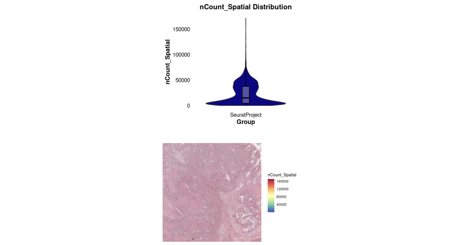
- 进一步处理,因为我这次处理的数据,是需要复现别人的结果,因此,我是没有自己再聚类(FindClusters)和注释的,直接用的别人注释好的文件
sp_obj <- SCTransform(sp_obj, assay = "Spatial", verbose = FALSE)  # 标准化
sp_obj <- RunPCA(sp_obj, assay = "SCT", verbose = FALSE)  # PCA
sp_obj <- FindNeighbors(sp_obj, reduction = "pca", dims = 1:30)  # 邻居查找
#sp_obj <- FindClusters(sp_obj, verbose = FALSE)  # 聚类,这里直接注释掉
sp_obj <- RunUMAP(sp_obj, reduction = "pca", dims = 1:30) # UMAP降维- 挂载别人注释好的文件
> head(sp_obj@meta.data)
                      orig.ident nCount_Spatial nFeature_Spatial nCount_SCT nFeature_SCT
AACACCTACTATCGAA-1 SeuratProject          90225            11403      15803         6494
AACACGTGCATCGCAC-1 SeuratProject           2638             1898      12580         5813
AACACTTGGCAAGGAA-1 SeuratProject          63980            10160      15590         6199
AACAGGAAGAGCATAG-1 SeuratProject           2956             2310      12369         5787
AACAGGATTCATAGTT-1 SeuratProject           2274             1539      13026         6160
AACAGGCCAACGATTA-1 SeuratProject           2161             1655      13554         6184
> load("ano_2.Rdata")
> head(ano_2)
              Barcode Cluster                      CellType
1  AACACCTACTATCGAA-1      11 Neuroendocrine_carcinoma_cell
5  AACACGTGCATCGCAC-1       4                   Fibroblasts
8  AACACTTGGCAAGGAA-1       1 Neuroendocrine_carcinoma_cell
12 AACAGGAAGAGCATAG-1       7                   Fibroblasts
14 AACAGGATTCATAGTT-1       4                   Fibroblasts
17 AACAGGCCAACGATTA-1       3                 Necrotic_cell
> table(rownames(sp_obj@meta.data) %in% ano_2$Barcode)

FALSE  TRUE
  101  4891
> # FALSE  TRUE
> # 101  4891
# 找出可以匹配的 spot
matched_barcodes <- intersect(rownames(sp_obj@meta.data), ano_2$Barcode)
# 过滤 Seurat 对象,只保留匹配的 spot
sp_obj <- subset(sp_obj, cells = matched_barcodes)

# 挂载 cluster 和 CellType 注释
matched_idx <- match(matched_barcodes, ano_2$Barcode)
sp_obj$Cluster <- ano_2$Cluster[matched_idx]
sp_obj$CellType <- ano_2$CellType[matched_idx]
# 检查
table(is.na(sp_obj$Cluster))  # 应该全部为 FALSE
table(is.na(sp_obj$CellType)) # 应该全部为 FALSE

metatada <- sp_obj@meta.data
metatada[1:2,]
table(metatada$CellType)

#一个 CellType 来自哪些 cluster
cluster_main_celltype <- table(metatada$Cluster, metatada$CellType)
write.csv(cluster_main_celltype,
file = "../SpatialAnalysisResults/1.数据概览/Sample#2/cluster_main_celltype.csv")- 可视化(因涉及到项目保密,只贴了空间聚类图)
# 可视化
#umap
pdf(file = file.path("../SpatialAnalysisResults/1.数据概览/Sample#2/umap_celltype.pdf"), width = 8.5, height = 6)
DimPlot(sp_obj, reduction = "umap", group.by = "CellType", label = TRUE,label.size = 4)
dev.off()
pdf(file = file.path("../SpatialAnalysisResults/1.数据概览/Sample#2/umap_cluster.pdf"), width = 7.5, height = 6)
DimPlot(sp_obj, reduction = "umap", group.by = "Cluster", label = TRUE)
dev.off()
#空间聚类CellType
pdf(file = file.path("../SpatialAnalysisResults/1.数据概览/Sample#2/Spatial_celltype_image.pdf"), width = 8.5, height = 6)
SpatialDimPlot(
  sp_obj,
  group.by = "CellType",
  pt.size.factor = 4.5,
  stroke = 0
) + theme(legend.position = "right")
dev.off()
pdf(file = file.path("../SpatialAnalysisResults/1.数据概览/Sample#2/Spatial_celltype.pdf"), width = 8.5, height = 6)
SpatialDimPlot(
  sp_obj,
  group.by = "CellType",
  pt.size.factor = 4.5,
  stroke = 0,
  image.alpha = 0#组织切片完全透明
) +
  theme(legend.position = "right")
dev.off()
#空间聚类Cluster
pdf(file = file.path("../SpatialAnalysisResults/1.数据概览/Sample#2/Spatial_cluster_image.pdf"), width = 7.5, height = 6)
SpatialDimPlot(
  sp_obj,
  group.by = "Cluster",
  pt.size.factor = 4.5,
  stroke = 0

) +
  theme(legend.position = "right")
dev.off()
pdf(file = file.path("../SpatialAnalysisResults/1.数据概览/Sample#2/Spatial_cluster.pdf"), width = 7.5, height = 6)
SpatialDimPlot(
  sp_obj,
  group.by = "Cluster",
  pt.size.factor = 4.5,
  stroke = 0,
  image.alpha = 0#组织切片完全透明
) +
  theme(legend.position = "right")
dev.off()

#只显示Adenocarcinoma_cell(腺癌细胞)与Adipocytes(脂肪细胞)
{

  sp_obj$CellType_highlight <- sp_obj$CellType
  sp_obj$CellType_highlight[
    !sp_obj$CellType %in% c("Adenocarcinoma_cell", "Adipocytes")
  ] <- "Other"

  cols <- c(
    "Adenocarcinoma_cell" = "#4575B4",
    "Adipocytes" = "#FDAE61",
    "Other" = "grey85"
  )

  pdf(file = file.path("../SpatialAnalysisResults/1.数据概览/Sample#2/Spatial_celltype_highlight.pdf"), width = 8.5, height = 6)
  SpatialDimPlot(
    sp_obj,
    group.by = "CellType_highlight",
    pt.size.factor = 4.5,
    stroke = 0,
    image.alpha = 0,
    cols = cols
  ) +
    theme(
      legend.position = "right",
      legend.title = element_blank()
    )
  dev.off()

  pdf(file = file.path("../SpatialAnalysisResults/1.数据概览/Sample#2/Spatial_celltype_highlight_image.pdf"), width = 8.5, height = 6)
  SpatialDimPlot(
    sp_obj,
    group.by = "CellType_highlight",
    pt.size.factor = 4.5,
    stroke = 0,
    cols = cols
  ) +
    theme(
      legend.position = "right",
      legend.title = element_blank()
    )
  dev.off()
}
sample2_sp_obj <- sp_obj
save(sample2_sp_obj,file = "../Rdata/step1_sample2_sp_obj.Rdata")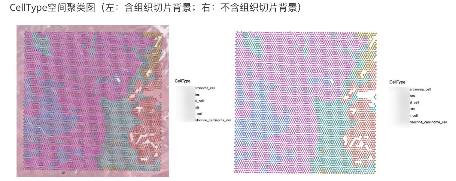
原创声明:本文系作者授权腾讯云开发者社区发表,未经许可,不得转载。
如有侵权,请联系 cloudcommunity@tencent.com 删除。
原创声明:本文系作者授权腾讯云开发者社区发表,未经许可,不得转载。
如有侵权,请联系 cloudcommunity@tencent.com 删除。
评论
登录后参与评论
推荐阅读
目录
腾讯云开发者

Copyright © 2013 - 2026 Tencent Cloud. All Rights Reserved. 腾讯云 版权所有
深圳市腾讯计算机系统有限公司 ICP备案/许可证号:粤B2-20090059 ![]() 粤公网安备44030502008569号
粤公网安备44030502008569号
腾讯云计算(北京)有限责任公司 京ICP证150476号 | 京ICP备11018762号