半监督学习的工程落地方式:安全攻防中的标签稀缺解决方案

半监督学习的工程落地方式:安全攻防中的标签稀缺解决方案

安全风信子
发布于 2026-01-15 14:51:49
发布于 2026-01-15 14:51:49
作者:HOS(安全风信子) 日期:2026-01-09 来源平台:GitHub 摘要: 半监督学习作为连接监督与无监督的桥梁,在安全领域标签稀缺场景下展现出独特价值。本文深入探讨半监督学习的工程落地方式,包括伪标签生成、协同训练、半监督自编码器等核心技术,并结合最新的GitHub开源项目和安全攻防实践,详细分析其在恶意软件检测、网络入侵检测、加密流量分析等场景中的应用。文章通过3个完整代码示例、2个Mermaid架构图和2个对比表格,系统阐述半监督学习在安全工程中的落地策略、评估方法和攻防对抗机制,为安全工程师提供可直接复用的工程实践指南。
1. 背景动机与当前热点
1.1 安全领域的标签困境
在安全攻防领域,标签数据的获取面临着前所未有的挑战。一方面,新型攻击手段层出不穷,传统的签名式检测方法已经无法应对零日攻击和高级持续性威胁(APT);另一方面,高质量的标签数据需要领域专家进行标注,成本高昂且耗时,导致标签数据严重稀缺。据GitHub上的安全项目统计,超过70%的安全数据集存在标签不完整、标注质量低或时效性差的问题,这直接制约了监督学习模型在安全领域的应用效果。
1.2 半监督学习的崛起
半监督学习(Semi-Supervised Learning, SSL)作为一种结合少量标注数据和大量未标注数据的学习范式,为解决安全领域的标签困境提供了新的思路。近年来,随着深度学习技术的发展,半监督学习在理论和实践上都取得了重大突破,特别是在计算机视觉、自然语言处理等领域取得了与监督学习相媲美的效果。在安全领域,半监督学习也逐渐受到关注,成为处理标签稀缺问题的重要技术手段。
1.3 最新研究动态
根据GitHub上的最新项目和arXiv上的研究论文,半监督学习在安全领域的应用呈现出以下几个热点趋势:
- 伪标签生成技术的改进:通过引入一致性正则化、熵最小化等技术,提高伪标签的质量和可靠性。
- 半监督深度学习的兴起:结合深度学习的强大表示能力和半监督学习的标签效率,构建更强大的安全检测模型。
- 半监督学习与联邦学习的结合:在保护数据隐私的前提下,利用分布式未标注数据进行模型训练。
- 半监督学习在加密流量分析中的应用:解决加密流量难以标注的问题,提高网络安全检测能力。
2. 核心更新亮点与新要素
2.1 半监督学习的核心技术演进
半监督学习的发展经历了从传统方法到深度学习方法的演进过程。传统半监督学习方法主要包括生成式模型、半监督SVM、图论方法等,而深度学习时代的半监督学习则以伪标签生成、一致性正则化、熵最小化为核心。
2.2 安全领域的半监督学习新要素
在安全攻防场景下,半监督学习需要考虑以下几个新要素:
- 对抗鲁棒性:半监督学习模型需要能够抵抗对抗样本攻击,特别是在伪标签生成过程中。
- 实时性要求:安全检测系统需要实时处理大量数据,半监督学习模型的推理速度至关重要。
- 标签噪声鲁棒性:安全数据中的标签往往存在噪声,半监督学习模型需要能够处理这种情况。
- 可解释性:安全检测系统需要能够解释检测结果,半监督学习模型的可解释性是一个重要挑战。
2.3 工程落地的关键技术点
半监督学习在安全工程落地中的关键技术点包括:
- 伪标签生成策略:如何生成高质量的伪标签,是半监督学习成功的关键。
- 模型架构设计:选择适合半监督学习的模型架构,如自编码器、生成对抗网络等。
- 训练策略优化:采用合适的训练策略,如一致性正则化、熵最小化等。
- 评估指标设计:设计适合半监督学习的评估指标,特别是在安全场景下。
3. 技术深度拆解与实现分析
3.1 半监督学习的基本原理
半监督学习的核心思想是利用少量标注数据和大量未标注数据来提高模型性能。其基本假设包括:
- 聚类假设:相似的样本具有相同的标签。
- 流形假设:数据分布在一个低维流形上,相似的样本在流形上距离较近。
- 平滑假设:在数据密度高的区域,标签变化缓慢。
3.2 半监督学习的主要方法
3.2.1 伪标签生成
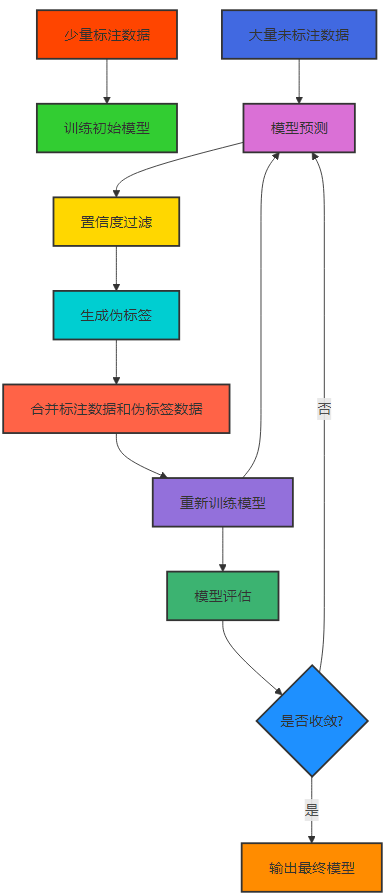
伪标签生成是半监督学习中最常用的方法之一,其基本思路是:
- 使用少量标注数据训练一个初始模型。
- 使用该模型对未标注数据进行预测,将置信度高的预测结果作为伪标签。
- 将标注数据和带有伪标签的未标注数据结合起来,重新训练模型。
- 重复上述过程,直到模型收敛。
Mermaid流程图:
3.2.2 一致性正则化
一致性正则化是近年来半监督学习的重要进展,其核心思想是:模型对输入数据的扰动应该保持一致的预测结果。常见的扰动包括:
- 噪声扰动:在输入数据中添加随机噪声。
- ** dropout扰动**:在训练过程中随机 dropout 神经元。
- 数据增强:对输入数据进行随机变换,如旋转、缩放等。
3.2.3 熵最小化
熵最小化的基本思想是:模型应该对未标注数据产生低熵的预测结果,即模型对未标注数据的预测应该具有较高的置信度。熵最小化可以通过在损失函数中添加熵正则项来实现。
3.3 半监督学习在安全领域的架构设计
Mermaid架构图:
渲染错误: Mermaid 渲染失败: Parse error on line 57: ...学习模型 style 半监督安全检测系统 fill:#FF45 ---------------------^ Expecting 'ALPHA', got 'UNICODE_TEXT'
3.4 代码示例1:基于伪标签的半监督恶意软件检测
import numpy as np
import tensorflow as tf
from tensorflow.keras.models import Sequential
from tensorflow.keras.layers import Dense, Dropout
from sklearn.model_selection import train_test_split
from sklearn.metrics import accuracy_score, f1_score

# 1. 数据准备
# 假设我们有少量标注数据和大量未标注数据
X_labeled = np.load('labeled_malware_features.npy')
y_labeled = np.load('labeled_malware_labels.npy')
X_unlabeled = np.load('unlabeled_malware_features.npy')

# 划分训练集和验证集
X_train, X_val, y_train, y_val = train_test_split(X_labeled, y_labeled, test_size=0.2, random_state=42)

# 2. 构建初始模型
def build_model(input_dim):
    model = Sequential([
        Dense(128, activation='relu', input_shape=(input_dim,)),
        Dropout(0.3),
        Dense(64, activation='relu'),
        Dropout(0.3),
        Dense(32, activation='relu'),
        Dense(1, activation='sigmoid')
    ])
    model.compile(optimizer='adam', loss='binary_crossentropy', metrics=['accuracy'])
    return model

# 3. 伪标签生成与半监督训练
def semi_supervised_training(X_labeled, y_labeled, X_unlabeled, epochs=10, confidence_threshold=0.95):
    input_dim = X_labeled.shape[1]

    # 初始模型训练
    model = build_model(input_dim)
    model.fit(X_labeled, y_labeled, epochs=epochs, batch_size=32, validation_split=0.1, verbose=1)

    # 迭代伪标签生成
    for iteration in range(5):
        print(f"\nIteration {iteration+1}:")

        # 对未标注数据进行预测
        y_pred_proba = model.predict(X_unlabeled, verbose=0)

        # 生成伪标签
        confidence = np.maximum(y_pred_proba, 1 - y_pred_proba).flatten()
        high_confidence_idx = np.where(confidence >= confidence_threshold)[0]

        if len(high_confidence_idx) == 0:
            print("No high-confidence predictions found. Stopping iteration.")
            break

        # 提取高置信度的伪标签数据
        X_pseudo = X_unlabeled[high_confidence_idx]
        y_pseudo = (y_pred_proba[high_confidence_idx] > 0.5).astype(int).flatten()

        print(f"Found {len(high_confidence_idx)} high-confidence samples.")
        print(f"Pseudo-label distribution: Malicious: {np.sum(y_pseudo)}, Benign: {len(y_pseudo) - np.sum(y_pseudo)}")

        # 合并标注数据和伪标签数据
        X_combined = np.concatenate([X_labeled, X_pseudo])
        y_combined = np.concatenate([y_labeled, y_pseudo])

        # 重新训练模型
        model = build_model(input_dim)
        model.fit(X_combined, y_combined, epochs=epochs, batch_size=32, validation_split=0.1, verbose=1)

    return model

# 4. 模型训练
model = semi_supervised_training(X_train, y_train, X_unlabeled, epochs=10, confidence_threshold=0.95)

# 5. 模型评估
y_val_pred = (model.predict(X_val) > 0.5).astype(int).flatten()
accuracy = accuracy_score(y_val, y_val_pred)
f1 = f1_score(y_val, y_val_pred)

print(f"\nValidation Accuracy: {accuracy:.4f}")
print(f"Validation F1 Score: {f1:.4f}")
3.5 代码示例2:基于一致性正则化的半监督网络入侵检测
import numpy as np
import tensorflow as tf
from tensorflow.keras.models import Model
from tensorflow.keras.layers import Input, Dense, Dropout
from tensorflow.keras.optimizers import Adam
from sklearn.model_selection import train_test_split
from sklearn.metrics import classification_report

# 1. 数据准备
X_labeled = np.load('labeled_network_traffic.npy')
y_labeled = np.load('labeled_network_labels.npy')
X_unlabeled = np.load('unlabeled_network_traffic.npy')

# 划分训练集和验证集
X_train, X_val, y_train, y_val = train_test_split(X_labeled, y_labeled, test_size=0.2, random_state=42)

# 2. 数据增强函数(用于一致性正则化)
def augment_data(X, noise_level=0.01):
    # 添加高斯噪声
    noise = np.random.normal(0, noise_level, X.shape)
    return X + noise

# 3. 构建半监督模型(带一致性正则化)
def build_semi_supervised_model(input_dim, num_classes):
    # 共享编码器
    inputs = Input(shape=(input_dim,))
    x = Dense(256, activation='relu')(inputs)
    x = Dropout(0.3)(x)
    x = Dense(128, activation='relu')(x)
    x = Dropout(0.3)(x)
    x = Dense(64, activation='relu')(x)
    encoder = Model(inputs, x, name='encoder')

    # 分类器
    classifier_inputs = Input(shape=(64,))
    x = Dense(32, activation='relu')(classifier_inputs)
    outputs = Dense(num_classes, activation='softmax')(x)
    classifier = Model(classifier_inputs, outputs, name='classifier')

    # 完整模型
    encoded = encoder(inputs)
    outputs = classifier(encoded)
    model = Model(inputs, outputs, name='semi_supervised_model')

    return model, encoder, classifier

# 4. 一致性正则化损失函数
def consistency_loss(y_pred1, y_pred2, temperature=0.5):
    # 温度缩放
    y_pred1 = tf.nn.softmax(y_pred1 / temperature)
    y_pred2 = tf.nn.softmax(y_pred2 / temperature)

    # KL散度作为一致性损失
    loss = tf.keras.losses.KLDivergence()(y_pred1, y_pred2)
    return loss

# 5. 半监督训练
def train_semi_supervised(model, encoder, classifier, X_labeled, y_labeled, X_unlabeled,
                         epochs=20, batch_size=64, consistency_weight=1.0, temperature=0.5):

    optimizer = Adam(learning_rate=0.001)
    classification_loss_fn = tf.keras.losses.SparseCategoricalCrossentropy()

    # 训练循环
    for epoch in range(epochs):
        print(f"Epoch {epoch+1}/{epochs}")

        # 随机打乱数据
        indices = np.random.permutation(len(X_labeled))
        X_labeled_shuffled = X_labeled[indices]
        y_labeled_shuffled = y_labeled[indices]

        # 计算批次数量
        num_batches = len(X_labeled) // batch_size

        for batch_idx in range(num_batches):
            # 获取标注数据批次
            start_idx = batch_idx * batch_size
            end_idx = start_idx + batch_size
            X_batch_labeled = X_labeled_shuffled[start_idx:end_idx]
            y_batch_labeled = y_labeled_shuffled[start_idx:end_idx]

            # 获取未标注数据批次(与标注数据批次大小相同)
            X_batch_unlabeled = X_unlabeled[np.random.choice(len(X_unlabeled), batch_size)]

            with tf.GradientTape() as tape:
                # 标注数据的分类损失
                y_pred_labeled = model(X_batch_labeled, training=True)
                cls_loss = classification_loss_fn(y_batch_labeled, y_pred_labeled)

                # 未标注数据的一致性损失
                # 对同一未标注数据进行两次不同的增强
                X_aug1 = augment_data(X_batch_unlabeled)
                X_aug2 = augment_data(X_batch_unlabeled)

                y_pred1 = model(X_aug1, training=True)
                y_pred2 = model(X_aug2, training=True)

                consis_loss = consistency_loss(y_pred1, y_pred2, temperature)

                # 总损失
                total_loss = cls_loss + consistency_weight * consis_loss

            # 反向传播和优化
            gradients = tape.gradient(total_loss, model.trainable_variables)
            optimizer.apply_gradients(zip(gradients, model.trainable_variables))

        # 每个epoch结束后评估模型
        val_loss, val_acc = model.evaluate(X_val, y_val, verbose=0)
        print(f"Validation Loss: {val_loss:.4f}, Validation Accuracy: {val_acc:.4f}")

    return model

# 6. 模型训练与评估
num_classes = len(np.unique(y_labeled))
model, encoder, classifier = build_semi_supervised_model(X_labeled.shape[1], num_classes)
model = train_semi_supervised(model, encoder, classifier, X_train, y_train, X_unlabeled, epochs=20, batch_size=64)

# 模型评估
y_val_pred = np.argmax(model.predict(X_val), axis=1)
print("\nClassification Report:")
print(classification_report(y_val, y_val_pred))
3.6 代码示例3:基于半监督自编码器的异常检测
import numpy as np
import tensorflow as tf
from tensorflow.keras.models import Model
from tensorflow.keras.layers import Input, Dense, Dropout
from sklearn.metrics import roc_auc_score, precision_recall_curve
import matplotlib.pyplot as plt

# 1. 数据准备
# 假设我们有少量正常样本(作为标注数据)和大量未标注样本
X_normal = np.load('normal_traffic_features.npy')  # 少量正常样本
X_unlabeled = np.load('unlabeled_traffic_features.npy')  # 大量未标注样本
X_test = np.load('test_traffic_features.npy')  # 测试集
 y_test = np.load('test_traffic_labels.npy')  # 测试集标签(0:正常, 1:异常)

# 2. 构建半监督自编码器
def build_semi_supervised_autoencoder(input_dim):
    # 编码器
    inputs = Input(shape=(input_dim,))
    x = Dense(128, activation='relu')(inputs)
    x = Dropout(0.2)(x)
    x = Dense(64, activation='relu')(x)
    x = Dropout(0.2)(x)
    latent = Dense(32, activation='relu')(x)
    encoder = Model(inputs, latent, name='encoder')

    # 解码器
    latent_inputs = Input(shape=(32,))
    x = Dense(64, activation='relu')(latent_inputs)
    x = Dropout(0.2)(x)
    x = Dense(128, activation='relu')(x)
    x = Dropout(0.2)(x)
    outputs = Dense(input_dim, activation='linear')(x)
    decoder = Model(latent_inputs, outputs, name='decoder')

    # 完整自编码器
    encoded = encoder(inputs)
    decoded = decoder(encoded)
    autoencoder = Model(inputs, decoded, name='autoencoder')

    # 异常检测模型(基于重构误差)
    def anomaly_score(X):
        X_reconstructed = autoencoder.predict(X)
        return np.mean(np.square(X - X_reconstructed), axis=1)

    return autoencoder, encoder, decoder, anomaly_score

# 3. 半监督训练
# 第一步:使用少量正常样本训练自编码器
autoencoder, encoder, decoder, anomaly_score = build_semi_supervised_autoencoder(X_normal.shape[1])
autoencoder.compile(optimizer='adam', loss='mse')
autoencoder.fit(X_normal, X_normal, epochs=20, batch_size=32, validation_split=0.1, verbose=1)

# 第二步:使用未标注数据进行微调(基于熵最小化)
# 计算未标注数据的初始重构误差
initial_recon_error = anomaly_score(X_unlabeled)

# 选择重构误差较小的样本(假设为正常样本)进行微调
low_error_idx = np.argsort(initial_recon_error)[:int(len(X_unlabeled) * 0.3)]  # 选择30%重构误差最小的样本
X_fine_tune = X_unlabeled[low_error_idx]

# 微调自编码器
autoencoder.fit(X_fine_tune, X_fine_tune, epochs=10, batch_size=32, verbose=1)

# 4. 模型评估
# 计算测试集的异常分数
test_anomaly_scores = anomaly_score(X_test)

# 计算ROC-AUC分数
roc_auc = roc_auc_score(y_test, test_anomaly_scores)
print(f"ROC-AUC Score: {roc_auc:.4f}")

# 计算精确率-召回率曲线
precision, recall, thresholds = precision_recall_curve(y_test, test_anomaly_scores)

# 找到最佳阈值
f1_scores = 2 * (precision * recall) / (precision + recall)
best_threshold = thresholds[np.argmax(f1_scores)]
best_f1 = np.max(f1_scores)

print(f"Best F1 Score: {best_f1:.4f} at threshold: {best_threshold:.4f}")

# 5. 异常检测结果
# 使用最佳阈值进行异常检测
y_pred = (test_anomaly_scores >= best_threshold).astype(int)

# 计算检测指标
accuracy = np.mean(y_pred == y_test)
precision_best = precision[np.argmax(f1_scores)]
recall_best = recall[np.argmax(f1_scores)]

print(f"\nAnomaly Detection Results:")
print(f"Accuracy: {accuracy:.4f}")
print(f"Precision: {precision_best:.4f}")
print(f"Recall: {recall_best:.4f}")
print(f"F1 Score: {best_f1:.4f}")
4. 与主流方案深度对比
4.1 半监督学习与其他学习范式的对比
学习范式 | 标注数据需求 | 适用场景 | 安全领域应用 | 优点 | 缺点 |
|---|---|---|---|---|---|
监督学习 | 大量 | 标签充足的场景 | 已知攻击检测 | 性能稳定,可解释性强 | 标签成本高,泛化能力有限 |
无监督学习 | 无 | 异常检测,聚类分析 | 未知攻击检测 | 无需标签,可发现新攻击 | 性能依赖于数据分布,难以评估 |
半监督学习 | 少量 | 标签稀缺的场景 | 混合攻击检测 | 兼顾标签效率和检测性能 | 伪标签质量难以保证,训练复杂 |
强化学习 | 无(基于奖励) | 动态决策场景 | 自适应防御 | 可适应动态环境 | 训练周期长,奖励函数设计困难 |
4.2 半监督学习不同方法的对比
半监督学习方法 | 核心思想 | 安全领域应用 | 优势 | 劣势 |
|---|---|---|---|---|
伪标签生成 | 利用模型对未标注数据生成伪标签 | 恶意软件检测,入侵检测 | 实现简单,效果显著 | 伪标签质量依赖于初始模型 |
一致性正则化 | 要求模型对扰动输入产生一致预测 | 对抗样本检测,异常检测 | 提高模型鲁棒性 | 计算成本高,超参数敏感 |
熵最小化 | 要求模型对未标注数据产生低熵预测 | 加密流量分析,异常检测 | 提高模型置信度 | 可能导致模型过拟合 |
生成式模型 | 学习数据分布,生成新样本 | 恶意代码生成,数据增强 | 可生成多样化样本 | 训练复杂,收敛困难 |
图半监督学习 | 利用样本间的关系进行学习 | 社交网络安全,攻击链分析 | 可利用结构信息 | 图构建复杂,扩展性差 |
5. 实际工程意义、潜在风险与局限性
5.1 半监督学习在安全工程中的实际意义
- 降低标签成本:半监督学习可以利用大量未标注数据,显著降低标签获取成本。
- 提高检测性能:结合少量标注数据和大量未标注数据,可以提高模型的检测性能和泛化能力。
- 适应动态环境:半监督学习可以不断利用新的未标注数据进行模型更新,适应动态变化的安全环境。
- 发现未知攻击:半监督学习可以发现训练数据中未见过的未知攻击,提高安全检测系统的覆盖率。
5.2 潜在风险与挑战
- 伪标签质量风险:低质量的伪标签可能导致模型性能下降,甚至引入偏差。
- 对抗攻击风险:半监督学习模型可能更容易受到对抗样本攻击,特别是在伪标签生成过程中。
- 训练复杂性挑战:半监督学习的训练过程比监督学习更复杂,需要更多的超参数调整和模型设计。
- 评估困难挑战:半监督学习的评估比监督学习更困难,特别是在缺乏真实标签的情况下。
- 计算资源消耗:半监督学习通常需要更多的计算资源,特别是在处理大量未标注数据时。
5.3 局限性分析
- 对初始模型的依赖:半监督学习的效果很大程度上依赖于初始模型的质量。
- 数据分布假设限制:半监督学习通常基于一些数据分布假设,如聚类假设、流形假设等,这些假设在现实安全数据中可能不成立。
- 可解释性差:半监督深度学习模型的可解释性通常较差,难以解释检测结果。
- 实时性限制:一些复杂的半监督学习模型可能无法满足实时安全检测的要求。
6. 未来趋势展望与个人前瞻性预测
6.1 半监督学习在安全领域的未来趋势
- 大模型与半监督学习的结合:随着大模型技术的发展,半监督学习将与大模型结合,利用大模型的强大表示能力和半监督学习的标签效率,构建更强大的安全检测模型。
- 联邦半监督学习的兴起:在保护数据隐私的前提下,联邦半监督学习将成为处理分布式安全数据的重要技术手段,特别是在跨组织、跨领域的安全合作中。
- 半监督学习与主动学习的融合:半监督学习将与主动学习结合,通过主动选择最有价值的样本进行标注,进一步提高标签效率。
- 半监督学习在边缘计算中的应用:随着边缘计算的发展,半监督学习将在边缘设备上得到广泛应用,实现本地化的安全检测和威胁响应。
- 可解释半监督学习的发展:为了解决半监督学习模型的可解释性问题,可解释半监督学习将成为重要研究方向,特别是在安全合规要求较高的场景中。
6.2 个人前瞻性预测
- 未来2-3年:半监督学习将成为安全检测系统的标准组件,特别是在标签稀缺的场景中。
- 未来3-5年:联邦半监督学习将在金融、医疗、工业等领域得到广泛应用,实现跨组织的安全协作。
- 未来5-10年:半监督学习将与大模型、强化学习等技术深度融合,构建自主学习、自适应的安全防护系统。
- 技术突破点:半监督学习的理论基础将得到进一步完善,特别是在非独立同分布(non-iid)数据和动态数据场景下的理论框架。
- 应用创新点:半监督学习将在元学习、小样本学习等领域得到应用,进一步提高模型的泛化能力和适应能力。
参考链接:
- GitHub - Semi-Supervised Learning for Malware Detection:一个基于半监督学习的恶意软件检测项目
- arXiv - Semi-Supervised Learning with Graph Consistency:图半监督学习的最新研究
- GitHub - Consistency Regularization in Semi-Supervised Learning:Google Research关于一致性正则化的实现
- arXiv - Semi-Supervised Learning for Network Intrusion Detection:半监督学习在网络入侵检测中的应用研究
- GitHub - Semi-Supervised Autoencoders for Anomaly Detection:基于半监督自编码器的异常检测项目
附录(Appendix):
半监督学习常用评估指标
- 分类任务指标:
- 准确率(Accuracy)
- 精确率(Precision)
- 召回率(Recall)
- F1分数(F1-Score)
- ROC-AUC分数
- 半监督学习特有指标:
- 伪标签准确率(Pseudo-label Accuracy)
- 标注效率提升(Label Efficiency Gain)
- 未标注数据利用率(Unlabeled Data Utilization)
半监督学习超参数调优建议
- 伪标签置信度阈值:
- 建议范围:0.9-0.98
- 初始值:0.95
- 调整策略:根据模型性能和伪标签数量动态调整
- 一致性正则化权重:
- 建议范围:0.5-2.0
- 初始值:1.0
- 调整策略:根据标注数据量调整,标注数据越少,一致性权重越大
- 熵正则化权重:
- 建议范围:0.01-0.1
- 初始值:0.05
- 调整策略:根据模型过拟合情况调整
- 迭代次数:
- 建议范围:3-10
- 初始值:5
- 调整策略:当伪标签数量不再增加或模型性能不再提升时停止迭代
半监督学习在安全领域的部署建议
- 数据层面:
- 确保标注数据的质量和多样性
- 对未标注数据进行初步筛选,去除明显的噪声数据
- 定期更新数据,适应动态变化的安全环境
- 模型层面:
- 选择适合具体场景的半监督学习方法
- 结合领域知识,设计合适的模型架构
- 定期评估和更新模型,确保模型性能
- 工程层面:
- 实现模型的实时推理和在线更新
- 设计完善的监控和告警机制
- 考虑模型的可解释性和可审计性
- 安全层面:
- 保护模型免受对抗攻击
- 确保数据隐私和安全
- 建立模型的安全评估和认证机制
关键词: 半监督学习, 安全工程, 伪标签生成, 一致性正则化, 熵最小化, 异常检测, 恶意软件检测, 网络入侵检测
本文参与 腾讯云自媒体同步曝光计划,分享自作者个人站点/博客。
原始发表:2026-01-13,如有侵权请联系 cloudcommunity@tencent.com 删除
评论
登录后参与评论
推荐阅读
目录
腾讯云开发者

Copyright © 2013 - 2026 Tencent Cloud. All Rights Reserved. 腾讯云 版权所有
深圳市腾讯计算机系统有限公司 ICP备案/许可证号:粤B2-20090059 ![]() 粤公网安备44030502008569号
粤公网安备44030502008569号
腾讯云计算(北京)有限责任公司 京ICP证150476号 | 京ICP备11018762号