病毒感染相关单细胞文献复现-1


❝文献标题:Single-cell sequencing of rotavirus-infected intestinal epithelium reveals cell-type specific epithelial repair and tuft cell infection. 杂志:Proc Natl Acad Sci U S A DOI: 10.1073/pnas.2112814118 ❞
文献简介
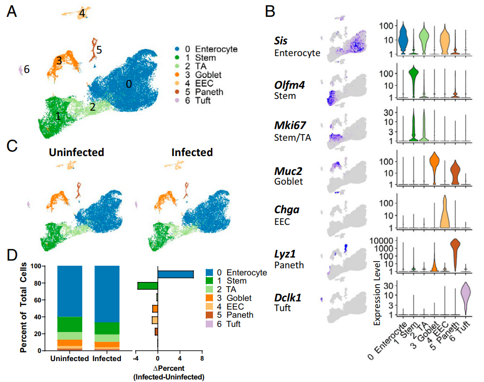
该篇文章重点研究了轮状病毒感染绒毛尖端的肠细胞会导致损伤。并且对感染的小鼠肠上皮进行的单细胞RNA测序显示了广泛的应答,包括干细胞扩增和不成熟的肠上皮细胞群。干细胞亚群更频繁地进入细胞周期,导致产生更多的肠上皮细胞来补偿绒毛尖端受损的肠上皮细胞。在丛状细胞中病毒转录物的存在和丛状细胞转录激活的证据表明丛状细胞在损伤后的上皮反应中提供了重要的信号。
复现的figure
常规的UMAP图+featureplot+小提琴图+分组UMAP图+细胞比例分布图
enterocyte, stem cell, transit amplifying cell [TA], goblet cell, EEC, Paneth cell, tuft cell
代码如下
step1-导入数据
rm(list=ls())
options(stringsAsFactors = F)
library(Seurat)
library(ggplot2)
library(clustree)
library(cowplot)
library(dplyr)
###### step1:导入数据 ######
library(stringr)
fs = list.files('./GSE169197/',pattern = '^GSM')
#执行这一步需要解压tar -xvf
samples=str_split(fs,'_',simplify = T)[,1]

lapply(unique(samples),function(x){
  y=fs[grepl(x,fs)]
  folder=paste0("GSE169197/", str_split(y[1],'_',simplify = T)[,1])
  dir.create(folder,recursive = T)
  #为每个样本创建子文件夹
  file.rename(paste0("GSE169197/",y[1]),file.path(folder,"barcodes.tsv.gz"))
  #重命名文件,并移动到相应的子文件夹里
  file.rename(paste0("GSE169197/",y[2]),file.path(folder,"features.tsv.gz"))
  file.rename(paste0("GSE169197/",y[3]),file.path(folder,"matrix.mtx.gz"))
})

dir='./GSE169197'
sceList = lapply(samples,function(pro){
  #pro=samples2[2]
  print(pro)
  sce =CreateSeuratObject(counts =  Read10X(file.path(dir,pro)) ,
                          project =  pro  ,
                          min.cells = 5,
                          min.features = 300 )
  return(sce)
})

sce.all=merge(x=sceList[[1]],
              y=sceList[-1])


library(stringr)
sce=sce.all
head(rownames(sce@meta.data))
tail(rownames(sce@meta.data))
table(sce$orig.ident)
sce$group<-ifelse(grepl("GSM5182802|5182805|5182807",sce$orig.ident),"Infected",
                   "Uninfected")
table(sce$group)

sce.all=sce
as.data.frame(sce.all@assays$RNA@counts[1:10, 1:2])
head(sce.all@meta.data, 10)
step2-常规QC(省略)
step3-降维分群
dir.create("2-harmony")
getwd()
setwd("2-harmony")

# sce.all=readRDS("../1-QC/sce.all_qc.rds")
sce=sce.all
sce
sce <- NormalizeData(sce,
                         normalization.method = "LogNormalize",
                         scale.factor = 1e4)
sce <- FindVariableFeatures(sce)
sce <- ScaleData(sce)
sce <- RunPCA(sce, features = VariableFeatures(object = sce))
step4-harmony及选择分辨率
#harmony
library(harmony)
seuratObj <- RunHarmony(sce, "orig.ident")
names(seuratObj@reductions)
seuratObj <- RunUMAP(seuratObj,  dims = 1:15,
                     reduction = "harmony")
DimPlot(seuratObj,reduction = "umap",label=T )

sce=seuratObj
sce <- FindNeighbors(sce, reduction = "harmony",
                     dims = 1:15)
sce.all=sce
#设置不同的分辨率,观察分群效果
for (res in c(0.01, 0.05, 0.1, 0.2, 0.3, 0.5,0.8,1)) {
  sce.all=FindClusters(sce.all,resolution = res, algorithm = 1)
}
colnames(sce.all@meta.data)

table(sce.all$orig.ident)
table(sce.all$group)

#接下来分析,按照分辨率为0.1进行
sel.clust = "RNA_snn_res.0.1"
sce.all <- SetIdent(sce.all, value = sel.clust)
table(sce.all@active.ident)
saveRDS(sce.all, "sce.all_int.rds")
getwd()
setwd('../')
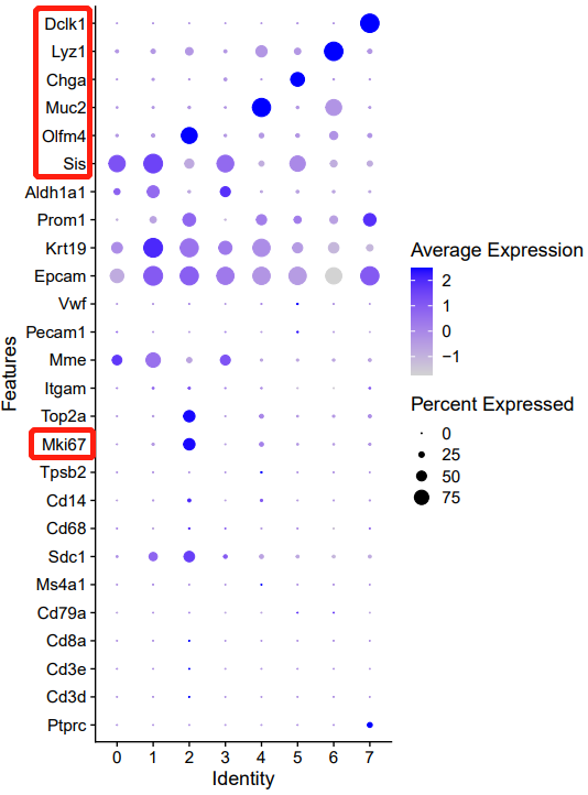
step5-根据常见marker gene 看分群
dir.create("3-cell")
setwd("3-cell/")
getwd()
sce.all=readRDS("../2-harmony/sce.all_int.rds")

DimPlot(sce.all, reduction = "umap", group.by = "seurat_clusters",label = T)
DimPlot(sce.all, reduction = "umap", group.by = "RNA_snn_res.0.1",label = T)
ggsave('umap_by_RNA_snn_res.0.1.pdf',width=6,height=5)
sce.all

library(ggplot2)
genes_to_check = c('PTPRC', 'CD3D', 'CD3E', 'CD4','CD8A','CD19', 'CD79A', 'MS4A1' ,
                   'IGHG1', 'MZB1', 'SDC1',
                   'CD68', 'CD163', 'CD14',
                   'TPSAB1' , 'TPSB2',  # mast cells,
                   'MKI67','TOP2A','KLRC1',
                   'RCVRN','FPR1' , 'ITGAM' ,
                   'FGF7','MME', 'ACTA2',
                   'PECAM1', 'VWF',
                   'KLRB1','NCR1', # NK
                   'EPCAM' , 'KRT19', 'PROM1', 'ALDH1A1',
                   'MKI67' ,'TOP2A',"SiS","OLFM4","MUC2","CHGA","LYZ1","DCLK1" )
library(stringr)
genes_to_check=str_to_title(unique(genes_to_check))
genes_to_check
p_all_markers <- DotPlot(sce.all, features = genes_to_check,
                         assay='RNA')  + coord_flip()

p_all_markers
ggsave(plot=p_all_markers, filename="check_all_marker_by_seurat_cluster.pdf",width=6,height=8)
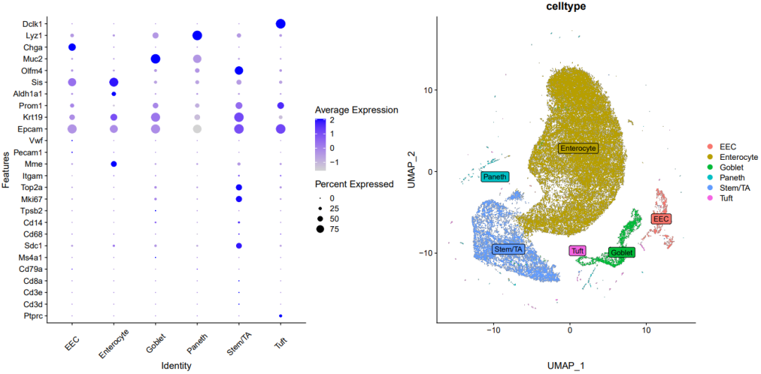
step6-细胞分群命名
rm(list=ls())
options(stringsAsFactors = F)
library(Seurat)
library(ggplot2)
library(clustree)
library(cowplot)
library(dplyr)
getwd()
# dir.create("3-cell")
setwd('3-cell/')
sce.all=readRDS( "../2-harmony/sce.all_int.rds")
sce.all

# 需要自行看图,定细胞亚群:
# 文章里面的 :
# enterocyte, stem cell,
# transit amplifying cell [TA],
# goblet cell, EEC,
# Paneth cell, tuft cell
celltype=data.frame(ClusterID=0:7,
                    celltype= 0:7)

#定义细胞亚群
celltype[celltype$ClusterID %in% c( 0,1,3 ),2]='Enterocyte'
celltype[celltype$ClusterID %in% c( 2),2]='Stem/TA'
celltype[celltype$ClusterID %in% c(4),2]='Goblet'
celltype[celltype$ClusterID %in% c( 5),2]='EEC'
celltype[celltype$ClusterID %in% c( 6),2]='Paneth'
celltype[celltype$ClusterID %in% c( 7),2]='Tuft'


head(celltype)
celltype
table(celltype$celltype)

sce.all@meta.data$celltype = "NA"
for(i in 1:nrow(celltype)){
  sce.all@meta.data[which(sce.all@meta.data$RNA_snn_res.0.1 == celltype$ClusterID[i]),'celltype'] <- celltype$celltype[i]}
table(sce.all@meta.data$celltype)


th=theme(axis.text.x = element_text(angle = 45,
                                    vjust = 0.5, hjust=0.5))

library(patchwork)
p_all_markers=DotPlot(sce.all, features = genes_to_check,
                      assay='RNA' ,group.by = 'celltype' )  + coord_flip()+th
p_umap=DimPlot(sce.all, reduction = "umap", group.by = "celltype",label = T,label.box = T)
p_all_markers+p_umap
ggsave('markers_umap_by_celltype.pdf',width = 16,height = 8)
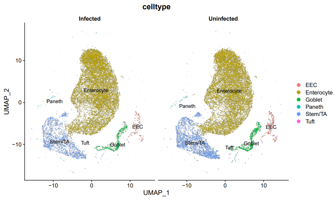
分组UMAP图
DimPlot(sce.all, reduction = "umap",split.by = 'group',
        group.by = "celltype",label = T)
ggsave('group_umap_RNA_snn_res.0.1.pdf',width = 10,height = 6)
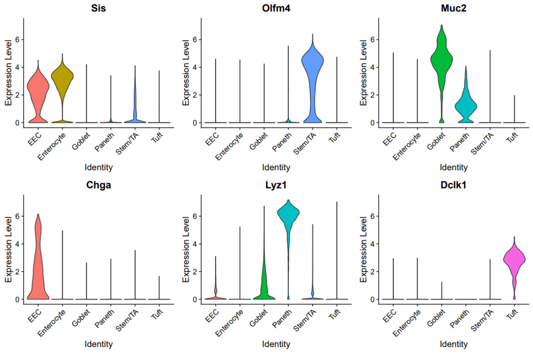
小提琴图
paper_marker=c("SiS","OLFM4","MUC2","CHGA","LYZ1","DCLK1")
library(stringr)
paper_marker=str_to_title(paper_marker)
paper_marker

p<-VlnPlot(sce.all, group.by = "celltype", features = paper_marker,
        pt.size = 0, ncol = 3, same.y.lims=T);p
ggsave(plot=p, filename="volin.pdf",width = 12,height = 8)
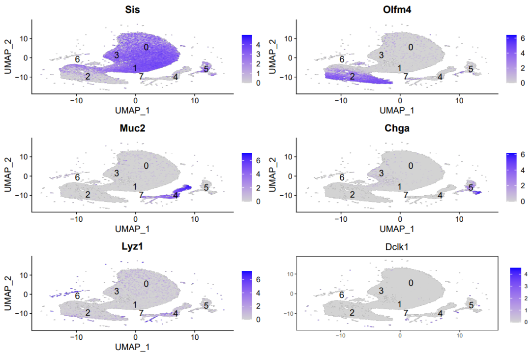
featureplot图
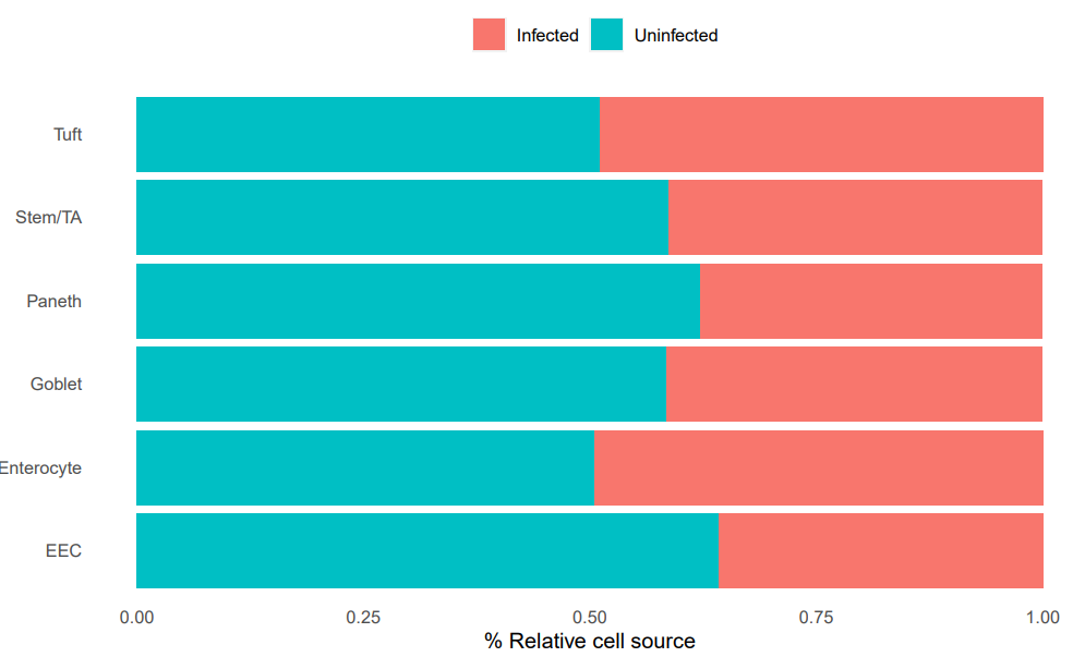
细胞亚群分布比例图
「我这里是按照分组展示不同的细胞亚群的分组比例」
phe=sce.all@meta.data
# 4.可视化 ----
## 4.1 每种细胞类型中,分组所占比例 ----
library(tidyr)# 使用的gather & spread
library(reshape2) # 使用的函数 melt & dcast
library(dplyr)
library(ggplot2)
tb=table(phe$celltype,
         phe$group)
head(tb)
bar_data <- as.data.frame(tb)

bar_per <- bar_data %>%
  group_by(Var1) %>%
  mutate(sum(Freq)) %>%
  mutate(percent = Freq / `sum(Freq)`)
head(bar_per)

#在这里替换X和fill的参数可以展示出和文章一样的效果~
ggplot(bar_per, aes(x =Var1 , y = percent)) +
  geom_bar(aes(fill = Var2) , stat = "identity") + coord_flip() +
  theme(axis.ticks = element_line(linetype = "blank"),
        legend.position = "top",
        panel.grid.minor = element_line(colour = NA,linetype = "blank"),
        panel.background = element_rect(fill = NA),
        plot.background = element_rect(colour = NA)) +
  labs(y = "% Relative cell source", fill = NULL)+labs(x = NULL)#+
  #scale_fill_d3()

ggsave("celltype_by_group_percent.pdf",
       units = "cm",width = 20,height = 12)
本文参与 腾讯云自媒体同步曝光计划,分享自微信公众号。
原始发表:2023-06-29,如有侵权请联系 cloudcommunity@tencent.com 删除
评论
登录后参与评论
推荐阅读
目录
腾讯云开发者

Copyright © 2013 - 2026 Tencent Cloud. All Rights Reserved. 腾讯云 版权所有
深圳市腾讯计算机系统有限公司 ICP备案/许可证号:粤B2-20090059 ![]() 粤公网安备44030502008569号
粤公网安备44030502008569号
腾讯云计算(北京)有限责任公司 京ICP证150476号 | 京ICP备11018762号