肝细胞癌(HCC)单细胞数据复现及解决上周推文的一些问题


❝肝细胞癌(HCC)是一种免疫治疗耐药的恶性肿瘤,具有高度的细胞异质性。人类和小鼠肝癌肿瘤的单细胞RNA测序揭示了癌症相关成纤维细胞(CAF)的异质性。今天复现的文献用了多个scRNA-seq测序,我这里选用人类的数据来做复现。 同时还有上周推文有一些错误的地方,这周推文后面做了解释,如果之后推文中有我不细心出现的错误欢迎大家指正! ❞
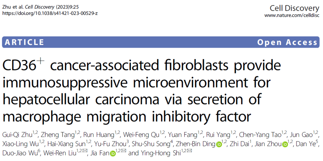
文献:
「cancer-associated fibroblasts provide immunosuppressive microenvironment for hepatocellular carcinoma via secretion of macrophage migration inhibitory factor.」 Cell Discov 2023 Mar 6;9(1):25.
数据集:
GEO Accession viewer (nih.gov)

step1 导入数据
rm(list=ls())
options(stringsAsFactors = F)
library(Seurat)
library(ggplot2)
library(clustree)
library(cowplot)
library(dplyr)

getwd()
# setwd("../")
###### step1:导入数据 ######
getwd()

library(stringr)
fs = list.files('./raw/',pattern = '^GSE')
#执行这一步需要解压tar -xvf
samples=str_split(fs,'_',simplify = T)[,1]

lapply(unique(samples),function(x){
  y=fs[grepl(x,fs)]
  folder=paste0("raw/", str_split(y[1],'_',simplify = T)[,1])
  dir.create(folder,recursive = T)
  #为每个样本创建子文件夹
  file.rename(paste0("raw/",y[1]),file.path(folder,"barcodes.tsv.gz"))
  #重命名文件,并移动到相应的子文件夹里
  file.rename(paste0("raw/",y[2]),file.path(folder,"features.tsv.gz"))
  file.rename(paste0("raw/",y[3]),file.path(folder,"matrix.mtx.gz"))
})

dir='./raw'

sce =CreateSeuratObject(counts =  Read10X("./raw/GSE202642/") ,
                        min.cells = 5,
                        min.features = 300 )
群里小伙伴上周发了一篇文献问能不能复现,并且群里小伙伴在处理数据的时候也遇到了一个问题。这里我来解答一下。
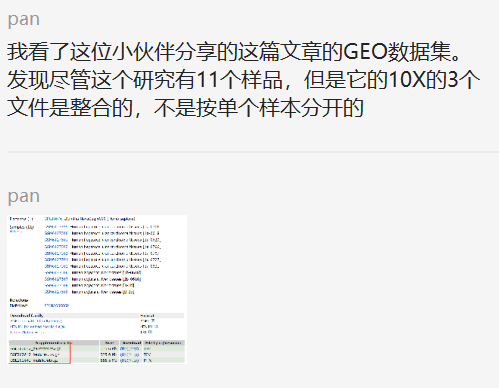
其实这个小知识点在之前的推文中有写过~分享一个小知识——单细胞转录组测序GSE数据集中sample是两个样本,而只有单个10X文件夹,这是为什么呢?
head(rownames(sce@meta.data))
tail(rownames(sce@meta.data))
phe=str_split(rownames(sce@meta.data),'-',simplify = T)
head(phe)
tail(phe)

sce@meta.data$orig.ident=paste0('p',phe[,2])
table(sce@meta.data$orig.ident)

sce$group<-ifelse(grepl("p8|9|10|11",sce$orig.ident),"Normal","HCCtumor")
table(sce$group)

sce.all=sce
as.data.frame(sce.all@assays$RNA@counts[1:10, 1:2])
head(sce.all@meta.data, 10)
tail(sce.all@meta.data, 10)
table(sce.all$orig.ident)
step2 QC步骤没有展示
step3 降维分群及harmony
 dir.create("2-harmony")
getwd()
setwd("2-harmony")

# sce.all=readRDS("../1-QC/sce.all_qc.rds")
sce=sce.all
sce
sce <- NormalizeData(sce,
                         normalization.method = "LogNormalize",
                         scale.factor = 1e4)
sce <- FindVariableFeatures(sce)
sce <- ScaleData(sce)
sce <- RunPCA(sce, features = VariableFeatures(object = sce))

library(harmony)
seuratObj <- RunHarmony(sce, "orig.ident")
names(seuratObj@reductions)
seuratObj <- RunUMAP(seuratObj,  dims = 1:15,
                     reduction = "harmony")
DimPlot(seuratObj,reduction = "umap",label=T )

sce=seuratObj
sce <- FindNeighbors(sce, reduction = "harmony",
                     dims = 1:15)
sce.all=sce
#设置不同的分辨率,观察分群效果(选择哪一个?)
for (res in c(0.01, 0.05, 0.1, 0.2, 0.3, 0.5,0.8,1)) {
  sce.all=FindClusters(sce.all, #graph.name = "CCA_snn",
                       resolution = res, algorithm = 1)
}

head(colnames(sce.all))
table(sce.all$orig.ident)
table(sce.all$group)

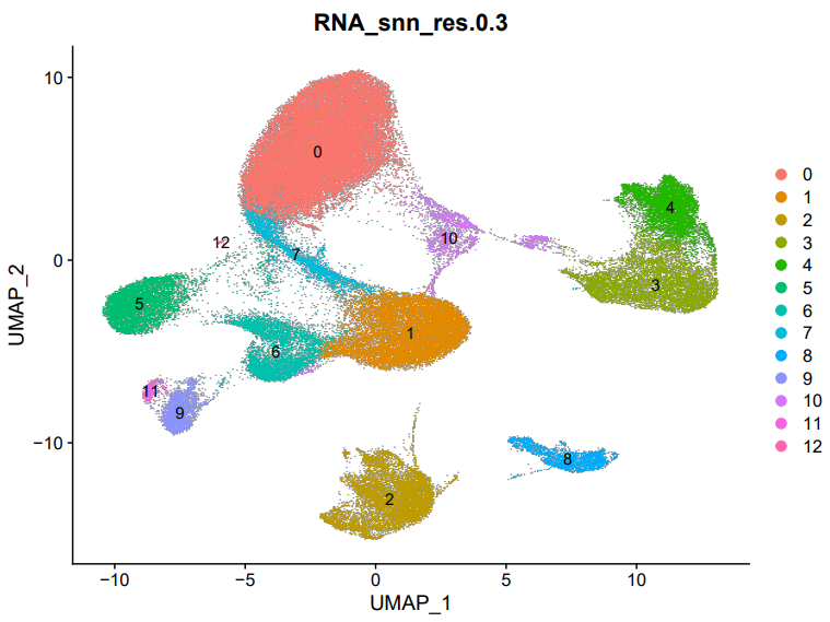
#接下来分析,按照分辨率为0.3进行
sel.clust = "RNA_snn_res.0.3"
sce.all <- SetIdent(sce.all, value = sel.clust)
table(sce.all@active.ident)
saveRDS(sce.all, "sce.all_int.rds")
getwd()
setwd('../')
step4 检查常见分群情况
dir.create("3-cell")
setwd("3-cell")
getwd()
#sce.all=readRDS("./2-harmony/sce.all_int.rds")

DimPlot(sce.all, reduction = "umap", group.by = "seurat_clusters",label = T)
DimPlot(sce.all, reduction = "umap", group.by = "RNA_snn_res.0.3",label = T)
ggsave('umap_by_RNA_snn_res.0.3.pdf',width = 8,height = 6)
library(ggplot2)
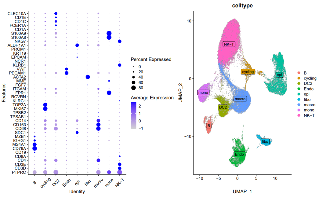
genes_to_check = c('PTPRC', 'CD3D', 'CD3E', 'CD4','CD8A','CD19', 'CD79A', 'MS4A1' ,
                   'IGHG1', 'MZB1', 'SDC1',
                   'CD68', 'CD163', 'CD14',
                   'TPSAB1' , 'TPSB2',  # mast cells,
                   'MKI67','TOP2A','KLRC1',
                   'RCVRN','FPR1' , 'ITGAM' ,
                   'FGF7','MME', 'ACTA2',
                   'PECAM1', 'VWF',
                   'KLRB1','NCR1', # NK
                   'EPCAM' , 'KRT19', 'PROM1', 'ALDH1A1',
                   'MKI67' ,'TOP2A',"NKG7","S100A8","S100A9" )
library(stringr)
genes_to_check=str_to_upper(unique(genes_to_check))
genes_to_check
p_all_markers <- DotPlot(sce.all, features = genes_to_check,
                         assay='RNA'  )  + coord_flip()
p_all_markers
ggsave(plot=p_all_markers, filename="check_all_marker_by_seurat_cluster.pdf",height = 11,width = 8)
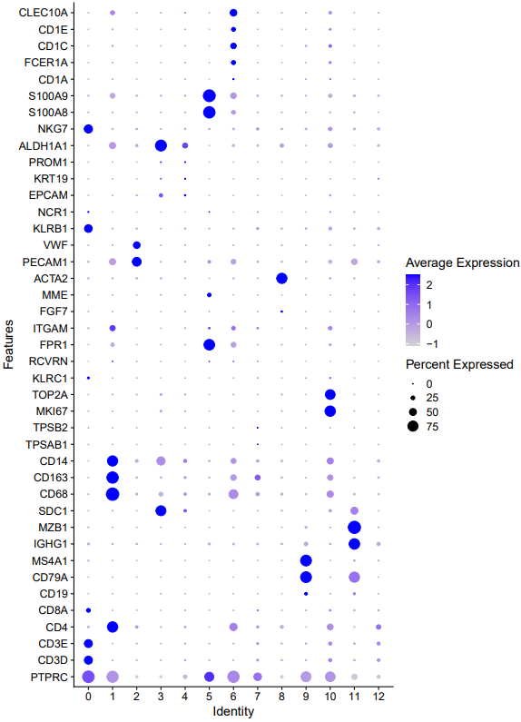
step5 定义细胞分群亚群
# 9,11:B
# 0,12:NK-T
# 1,7:Mac
# 6:DC2
# 5:   Mono
# 2: Endo
# 3,4: epi
# 10: cycling
# 8:fibo

celltype=data.frame(ClusterID=0:12,
                    celltype= 0:12)

#定义细胞亚群
celltype[celltype$ClusterID %in% c(9,11 ),2]='B'
celltype[celltype$ClusterID %in% c( 0,12),2]='NK-T'
celltype[celltype$ClusterID %in% c(2),2]='Endo'
celltype[celltype$ClusterID %in% c( 10 ),2]='cycling'
celltype[celltype$ClusterID %in% c( 1,7),2]='macro'
celltype[celltype$ClusterID %in% c( 5),2]='mono'
celltype[celltype$ClusterID %in% c(3,4),2]='epi'
celltype[celltype$ClusterID %in% c(8),2]='fibo'
celltype[celltype$ClusterID %in% c(6),2]='DC2'

head(celltype)
celltype
table(celltype$celltype)

sce.all@meta.data$celltype = "NA"
for(i in 1:nrow(celltype)){
  sce.all@meta.data[which(sce.all@meta.data$RNA_snn_res.0.3 == celltype$ClusterID[i]),'celltype'] <- celltype$celltype[i]}
table(sce.all@meta.data$celltype)

th=theme(axis.text.x = element_text(angle = 45,
                                    vjust = 0.5, hjust=0.5))
library(patchwork)
p_all_markers=DotPlot(sce.all, features = genes_to_check,
                      assay='RNA' ,group.by = 'celltype' )  + coord_flip()+th
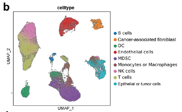
p_umap=DimPlot(sce.all, reduction = "umap", group.by = "celltype",label = T,label.box = T)
p_all_markers+p_umap
ggsave('markers_umap_by_celltype_2.pdf',width = 13,height = 8)
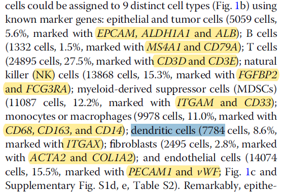
「文章中的marker gene」
「对比文章中的umap图」
关于上周推文的一些问题


- 在此更正:腹主动脉瘤不是一种肿瘤,虽然叫瘤,但是是一种血管畸形疾病,不是肿瘤。
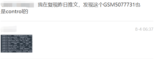
- 对照组有两个样本,所以我在做分组的umap图的时候做错了。 在此更正:
sce$group<-ifelse(grepl("GSM5077732|GSM5077731",sce$orig.ident),"Control","Tumor")
table(sce$group)
本文参与 腾讯云自媒体同步曝光计划,分享自微信公众号。
原始发表:2023-08-10,如有侵权请联系 cloudcommunity@tencent.com 删除
目录
腾讯云开发者

Copyright © 2013 - 2026 Tencent Cloud. All Rights Reserved. 腾讯云 版权所有
深圳市腾讯计算机系统有限公司 ICP备案/许可证号:粤B2-20090059  粤公网安备44030502008569号
腾讯云计算(北京)有限责任公司 京ICP证150476号 | 京ICP备11018762号