Matplotlib数据分布型图表(1)

Matplotlib数据分布型图表(1)

python数据可视化之路
发布于 2023-02-23 20:52:32
发布于 2023-02-23 20:52:32
数据分布图表主要显示数据集中的数值及其出现的频率或者分布规律,包括统计直方图、核密度曲线图、箱型图、小提琴图等。其中,统计直方图最为简单和常见,又称质量分布图,由一系列高度不等的纵向条纹或线段表示数据分布的情况。一般横轴表示数据类型,纵轴表示数据情况。
1 统计直方图
统计直方图类似柱状图,但是与柱状图相比有不同含义。统计直方图的作用:1)能够显示各组的频数或数量分布情况;2)易于显示各组之间的频数或数量差别,通过直方图可以看出哪些数据比较集中或者孤立的数据分布。
现有一组数据,记录了2015年全国各站点的PM2.5浓度值,现用统计直方图表示。

相关语法为
plt.hist(x,bins=None,range=None,density=None,log=False,**kwargs)
x:需要统计的数组
bins:分组数。就是传入的数组需要划分为几部分。
range:x轴的范围。
density:是否设置y轴为密度(默认为每一组中的数据个数)。
log:是否设置y轴为对数格式,默认为False。
**kwargs:其他参数设置,例如color,edgecolor和alpha。
代码如下:
import pandas as pd
import matplotlib.pyplot as plt
import matplotlib as mpl
mpl.rcParams['font.sans-serif'] = ['Times New Roman'] #设置默认字体

#构造数据
file = r"D:\公众号\Pandas基本操作\2015预测.csv"
df = pd.read_csv(file)
x = df['pm2_5'].values
x = x[x <= 400] #选择pm2.5小于400的数值

fig = plt.figure(figsize = (8, 12))

#默认绘图,设置20个分组,线框颜色为黑色,与ax5共享x轴,设置x轴刻度为空
ax1 = fig.add_subplot(321, sharex = ax5)
ax1.hist(x, bins = 20, edgecolor = 'k')
ax1.set_xticks([])

#设置x轴范围,并利用对数表示y轴刻度
ax2 = fig.add_subplot(322, sharex = ax5)
ax2.hist(x, bins = 20, edgecolor = 'k', range = (0, 300), log = True)
ax2.set_xticks([])

#设置y轴为密度轴,并设置y轴刻度
ax3 = fig.add_subplot(323, sharex = ax5)
ax3.hist(x, bins = 20, range = (0, 300), density = True, edgecolor = 'k')
ax3.set_xticks([])
ax3.set_yticks(np.arange(0, 0.021, 0.005))

#在ax3基础上添加密度线
ax4 = fig.add_subplot(324, sharex = ax5, sharey = ax3)
n2, bins2, patches2 = ax4.hist(x, bins=50, range = (0, 300), density = True)
ax4.plot(bins2[:-1], n2, linestyle = '--', lw = 3, color = 'r')
ax4.set_xticks([])

#设置cumulative参数从而将密度线样式为累加线
ax5 = fig.add_subplot(313)
n2, bins2, patches2 = ax5.hist(x, bins=50, range = (0, 300), edgecolor = 'k', density = True, cumulative=True, alpha = 0.5)
ax5.plot(bins2[:-1], n2, linestyle = '--', lw = 3, color = 'r')

#适当调整子图的横纵间距
plt.subplots_adjust(wspace = 0.20, hspace = 0.08)
plt.show()
2 核密度估计图
核密度估计图用于显示数据在x轴连续数据的分布状况,它是统计直方图的变种,使用平滑曲线绘制数据水平,从而得出更光滑的分布。核密度估计图比统计直方图优胜的地方在,它不受使用分组数量的影响,所以能更好的界定分布形状。
虽然在以上统计直方图中绘制了密度图,这里介绍另外一种绘制方法——利用seaborn库的distplot函数。
注:在displot函数中,默认绘制密度线,即kde = True;默认绘制直方图,即hist = True。
代码如下(利用前面的数据):
import seaborn as sns
fig = plt.figure(figsize = (8, 4))
#设置密度线的样式
ax1 = fig.add_subplot(121)
sns.distplot(x, bins = 20, kde_kws = {'color':'r', 'linestyle': '--'}, ax = ax1)
ax1.set_yticks(np.arange(0, 0.02, 0.005))
#设置直方图的样式
ax2 = fig.add_subplot(122)
sns.distplot(x, bins = 20, hist_kws = {'edgecolor':'k'}, kde_kws = {'color':'r', 'linestyle': '--'}, ax = ax2)
ax2.set_yticks(np.arange(0, 0.02, 0.005))

plt.show()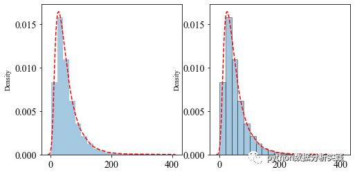
本文参与 腾讯云自媒体同步曝光计划,分享自微信公众号。
原始发表:2022-06-18,如有侵权请联系 cloudcommunity@tencent.com 删除
腾讯云开发者

Copyright © 2013 - 2026 Tencent Cloud. All Rights Reserved. 腾讯云 版权所有
深圳市腾讯计算机系统有限公司 ICP备案/许可证号:粤B2-20090059  粤公网安备44030502008569号
腾讯云计算(北京)有限责任公司 京ICP证150476号 | 京ICP备11018762号