跟着NBT学做图：样本地理信息图

小汪Waud

发布于 2023-02-20 11:34:30

1.3K0

今天我们来学习一下刘永鑫老师2019年发表在Nature Biotechnology上的文章NRT1.1B is associated with root microbiota composition and nitrogen use in field-grown rice中的代码。

其代码和数据都已经在其github[1]免费分享，按下图操作即可全部打包。下载缓慢的朋友也可在公众号回复「20220902」获得压缩包。

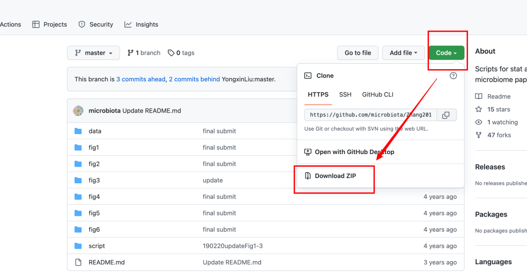
https://github.com/microbiota/Zhang2019NBT

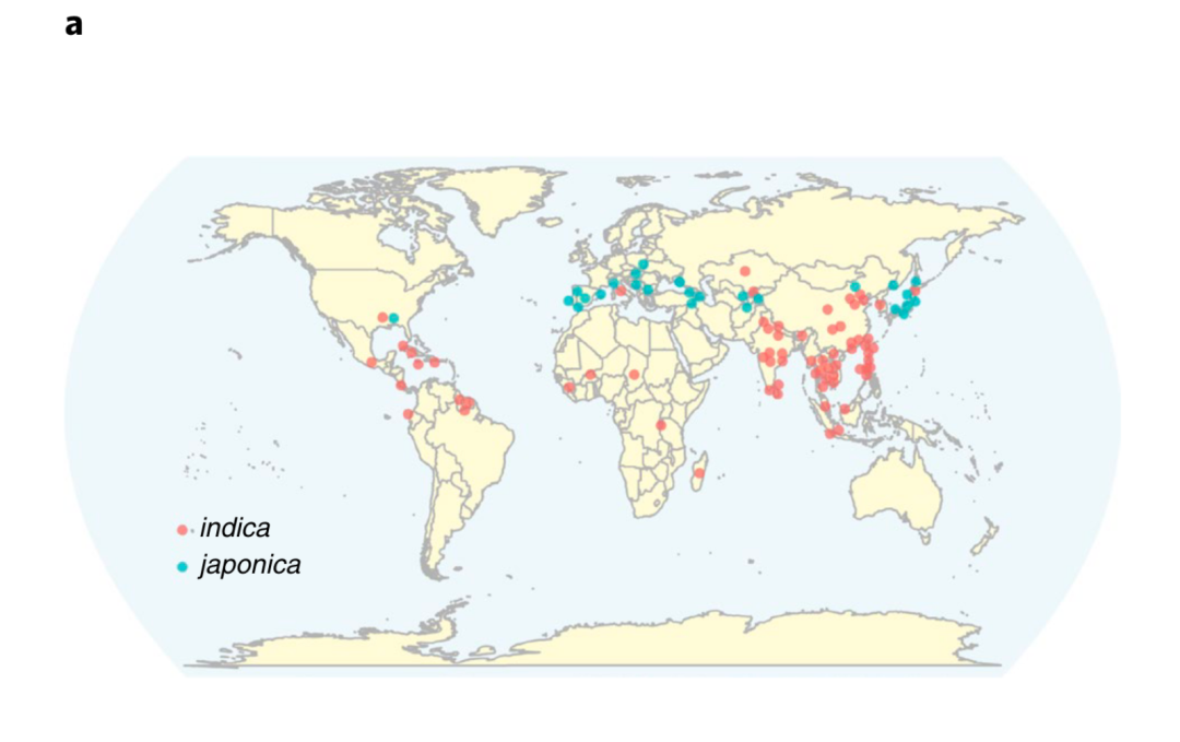
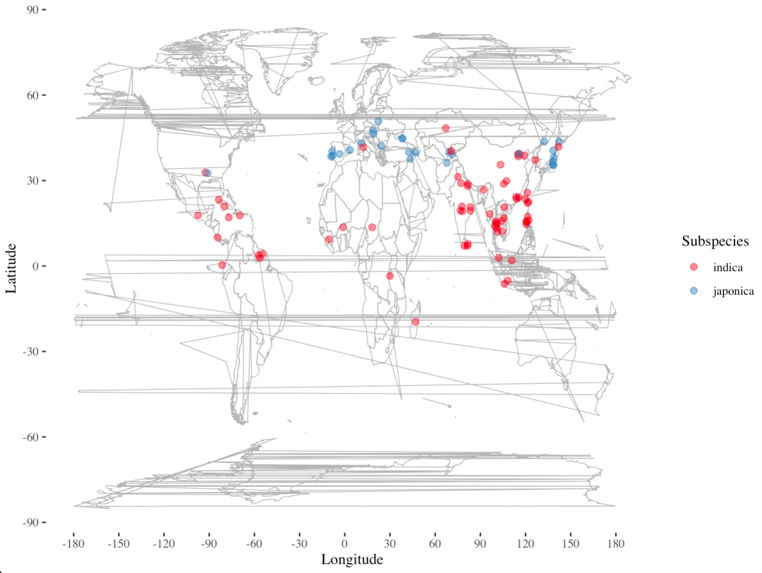
图1 a Diagram of original collection sites (44 countries) of indica (red) and japonica (blue) rice

图1 a主要介绍了本研究中样本籼稻（indica）和粳稻（japonica）的位置。

源代码

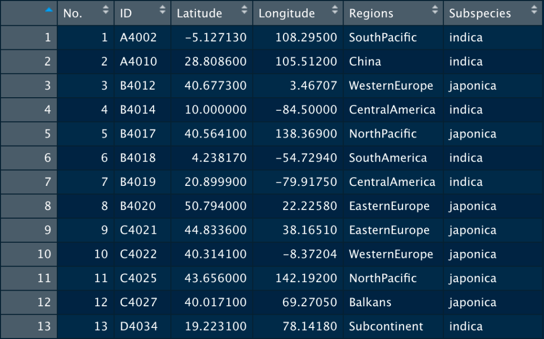
在作图之前我们需要准备「包含样本地理位置信息的表」，至少包含品种和经纬度。

首先我放上经过我详细注释后的代码。

library(dplyr)
library(maptools)
library(ggthemes)
library(ggplot2)
library(maps)

geotable = read.table("varieties_geo.txt", header = T, sep = "\t") # 读取地理信息
worldmap = map_data("world") # 引入世界地图数据
# 通过?map_data查看，仅能提供county,france,italy,nz,state,usa,world,world2等几款地图

fig1 = ggplot(geotable, aes(Longitude, Latitude, color = Subspecies)) +
  geom_polygon(data = worldmap, aes(x = long, y = lat, group = group, fill = NA), 
               color = "grey70", size = 0.25)+ # 绘制地图
  geom_point(size = 2, alpha = 0.5)+ # 绘制具体的位置点
  scale_colour_brewer(palette = "Set1") + # 设置主题颜色
  scale_fill_brewer(palette = "Set1")+  # 设置主题颜色
  scale_y_continuous(breaks = (-3:3)*30)+ # 将Y轴的刻度限制为-90～90
  scale_x_continuous(breaks = (-6:6)*30)+ # 将X轴的刻度限制为-180～180
  labs(x="Longitude", y="Latitude", colour = "Subspecies" ) + # 修改X轴、Y轴及图例
  theme_tufte() # 需要library(ggthemes)
fig1
ggsave(paste0(output_dir, "minicore-worldmap.pdf", sep=""), fig1, width = 9, height = 5)

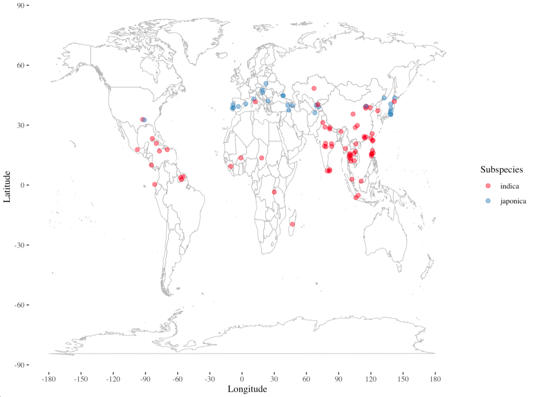
源代码出的图

函数详解

map_data()

map_data()[2]是ggplot2的一个函数，用于将map包中的数据转换为适合ggplot2绘图的框架。

「主要用法」

map_data(map, region = ".", exact = FALSE, ...)

「主要参数」

map：可以提供的地图，包括county(United States County Map), france,italy, nz(New Zealand Basic Map),state(United States State Boundaries Map), usa(United States Coast Map), world(Low (mid) resolution World Map), world2(Pacific Centric Low resolution World Map)。
region：包含子区域的名称，默认包含所有子区域。
exact：将region视为正则表达式(FALSE)还是固定字符串(TRUE)。

「示例」

library(ggplot2)
states <- map_data("state") # 引入美国地图
arrests <- USArrests
names(arrests) <- tolower(names(arrests)) # 将arrests的列名改为小写
arrests$region <- tolower(rownames(USArrests)) # 将USArrests的行名转换为小写并作为新增的一列保存为region，用于后续合并

choro <- merge(states, arrests, sort = FALSE, by = "region") # 通过region合并states和arrests
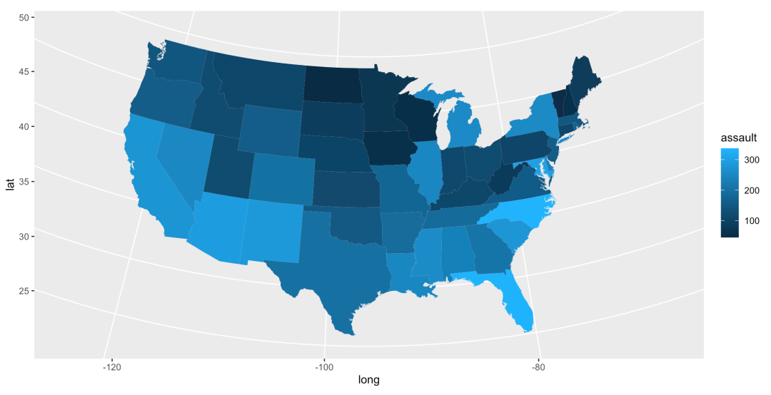
ggplot(choro, aes(long, lat)) + # 根据经纬度绘制地图
  geom_polygon(aes(group = group, fill = assault)) +
  coord_map("albers", lat0 = 45.5, lat1 = 29.5) 
# coord_map() 将地球的一部分近似球面投影到一个平面的2D平面上
# albers(lat0,lat1)：equal-area, true scale on lat0 and lat1

USArrests[3]包含了1973年美国50个州每10万居民中因袭击(assault)、谋杀(murder)和强奸(rap)而被捕的人数，还给出了生活在城市地区的人口百分比(urbanpop，Percent urban population)。

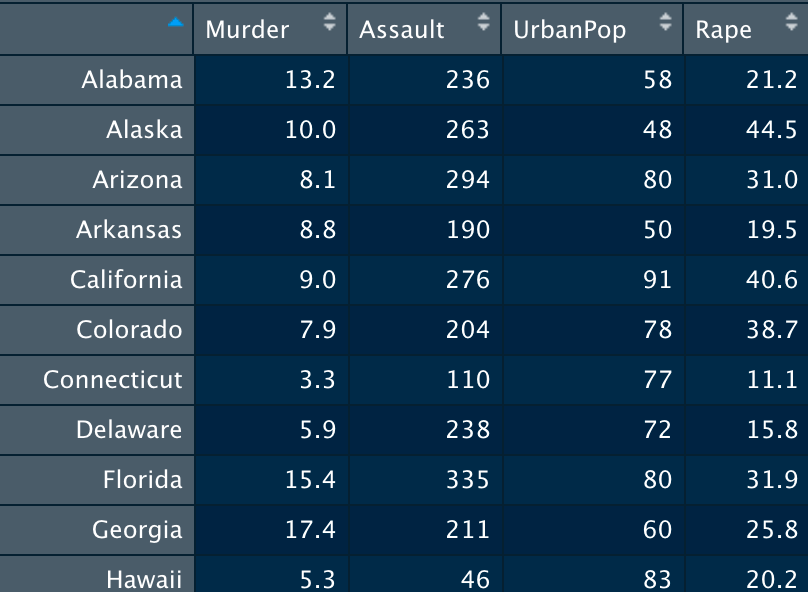
arrests

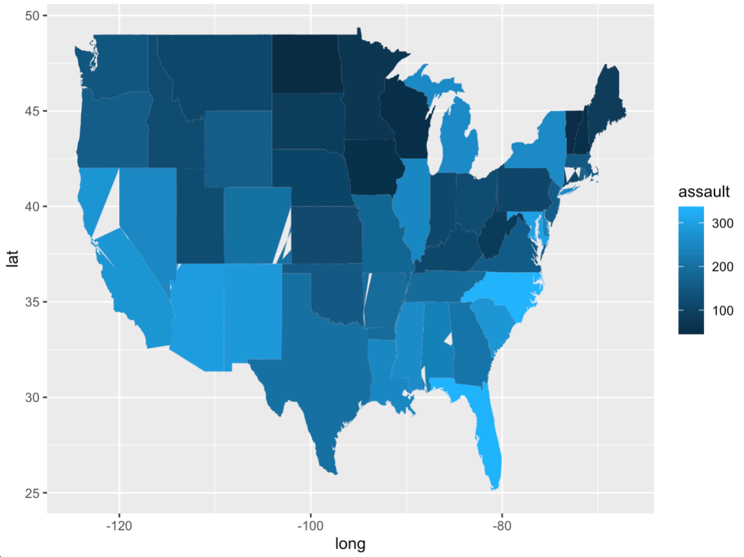
不添加coord_map("albers", lat0 = 45.5, lat1 = 29.5)

geom_polygon()

geom_polygon()[4]非常类似于由geom_path()绘制的路径，只不过起始点和结束点相连，内部可以填充。group映射决定了哪些case被连接在一起成为一个多边形。

「主要用法」

geom_polygon(
  mapping = NULL,
  data = NULL,
  stat = "identity",
  position = "identity",
  rule = "evenodd",
  ...,
  na.rm = FALSE,
  show.legend = NA,
  inherit.aes = TRUE)

「主要参数」

mapping：同ggplot2
data：同ggplot2
stat：使用的统计转换
position：位置调整
rule：可选evenodd或winding，如果要绘制带孔的多边形，这个参数定义了如何解释孔的坐标，示例[5]。
na.rm：默认情况下（False），缺失值会被移除并警告；选择True，缺失值会被悄无声息的移除。
show.legend：默认不展示。
inherit.aes：如果选择False，将会覆盖默认的映射（aesthetics），而不是将它们结合。

「注意⚠️」

在源代码中，关于geom_polygon的参数group，有一点需要注意。

geom_polygon(data = worldmap, aes(x = long, y = lat, group = group, fill = NA), 
               color = "grey70", size = 0.25)

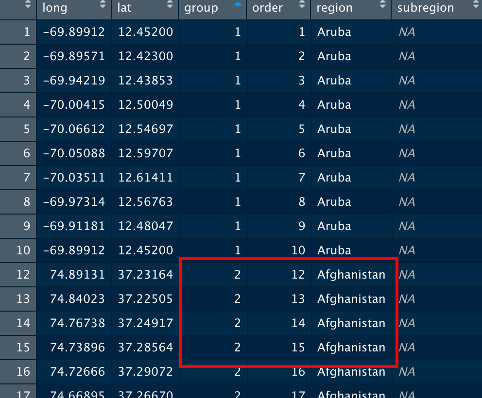
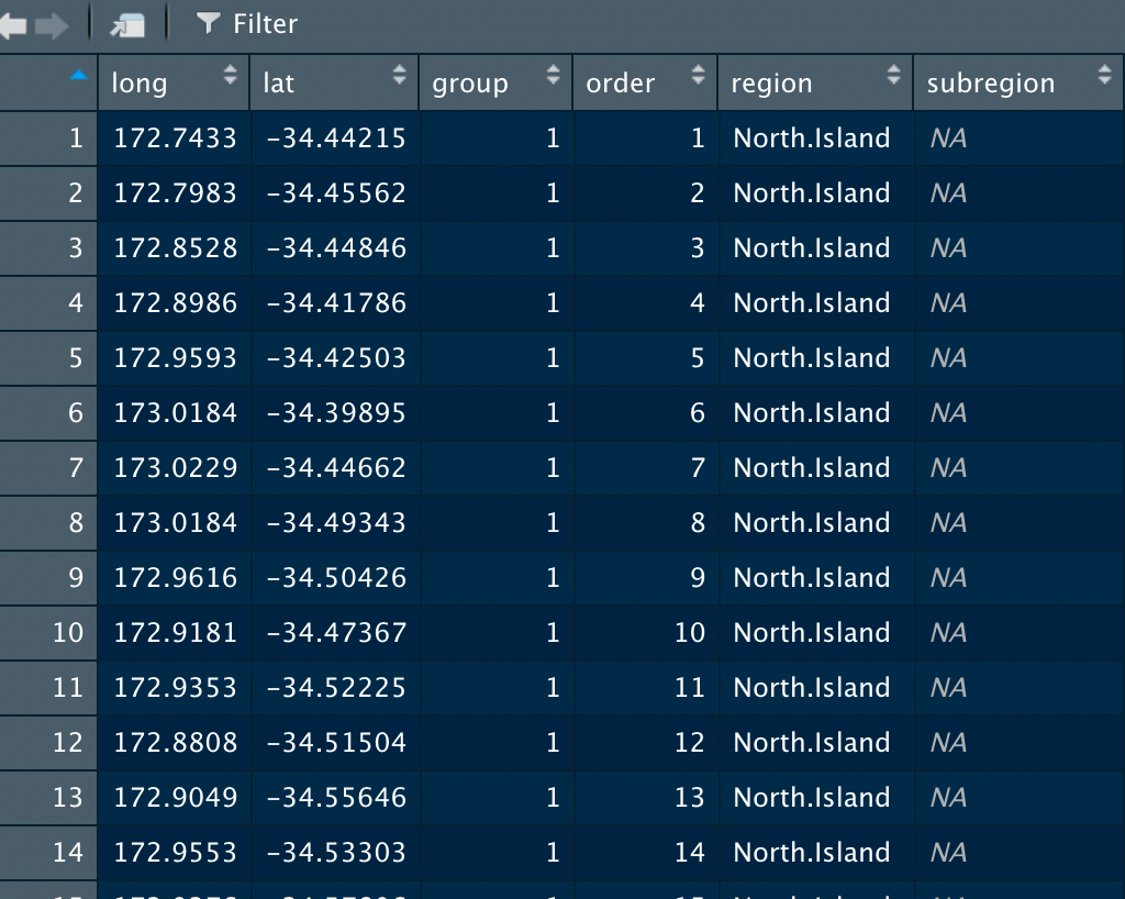
worldmap

在这里group=group，而观察后我们发现，每个region对应了一个group，比如Aruba对应group 1，Afghanistan对应group 2，enclave对应group 1627，既然这样，能否group=region呢？

group=region

此时你应该明白，地图数据中的group是有意义的，决定了连线的先后顺序，在其他地图包中也有该顺序。

New Zealand Basic Map

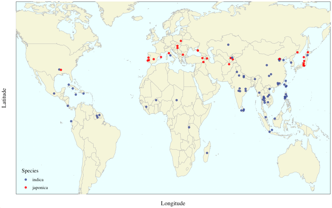
美化

我对代码进行了微调，包括地图背景颜色、字/点的大小、透明度，把图限制在了一定区间范围，同时修改了主题。

library(dplyr)
library(maptools)
library(ggthemes)
library(ggplot2)
library(maps)
library(ggsci)
geotable = read.table("varieties_geo.txt", header = T, sep = "\t") # 读取地理信息
worldmap = map_data("world") # 引入世界地图数据
# 通过?map_data查看，仅能提供county,france,italy,nz,state,usa,world,world2等几款地图

fig = ggplot(geotable, aes(Longitude, Latitude, color = Subspecies)) +
  geom_polygon(data = worldmap, aes(long, lat, group = group, fill = NA), 
               color = "grey70",fill = "#F5F5DC", size = 0.25) + # 绘制地图
  geom_point(size = 1.7, alpha = 0.8)+ # 绘制具体的位置点
  labs(x="Longitude", y="Latitude", color = "Species" ) + # 修改X轴、Y轴及图例
  coord_cartesian(xlim = c(-120,150), ylim = c(-40,70)) +
  theme_tufte() + # 需要library(ggthemes) 
  theme(axis.ticks = element_line(linetype = "blank"), # 去掉坐标轴
  axis.text = element_text(colour = NA), # 去掉坐标轴的数字标记
  panel.background = element_rect(fill = '#F0FFFF'), # 背景色
  axis.title = element_text(size = 13),
  legend.text = element_text(size = 10),
  legend.title = element_text(size = 12),
  legend.position = c(0.06, 0.075)) + # 修改图例位置
  scale_color_aaas() # 修改主题 
 
fig

如果你用上了他们的代码，请务必按照下列方法引用：

Jingying Zhang#, Yong-Xin Liu#, Na Zhang#, Bin Hu#, Tao Jin#, Haoran Xu, Yuan Qin, Pengxu Yan, Xiaoning Zhang, Xiaoxuan Guo, Jing Hui, Shouyun Cao, Xin Wang, Chao Wang, Hui Wang, Baoyuan Qu, Guangyi Fan, Lixing Yuan, Ruben Garrido-Oter, Chengcai Chu* & Yang Bai*. NRT1.1B is associated with root microbiota composition and nitrogen use in field-grown rice. Nature Biotechnology. 2019. doi:10.1038/s41587-019-0104-4